In bulk isotropic superconductors at low temperatures, vortices can be
accurately modeled as perfectly rigid rods aligned with the
externally applied magnetic field [1].
In an anisotropic material, such as the layered superconductor
Bi2Sr2CaCu2Ox,
at high enough temperatures the vortices no longer appear rigid but are
instead broken up into disk-like "pancake vortices," one per layer,
with an attractive interaction between pancakes in adjacent layers
along the length of the vortex
[2,3,4,5,6]. In
this case, the fully three-dimensional nature of
the vortex must be taken into account when studying
the interaction of vortices and pinning sites.
An understanding of layered materials is important because many
high-temperature superconductors have a layered structure, including
YBa2Cu3O7−δ
[7,8,9],
Bi2Sr2CaCu2Ox
[10,11],
and
Tl-cuprate superconductors [12,13,14]
The degree of anisotropy in these materials varies,
causing the three-dimensional nature of the
vortex to be of greater or lesser importance.
In each case, however, the two-dimensional approximation
for the flux line used in the simulations described
in [1] is inadequate.
The interactions between vortices and different types of pinning centers,
and the resulting effect on the critical current of the anisotropic material,
is not yet completely understood. Artificially created pins, such
as point or columnar pins, strongly affect the vortex behavior
and can further enhance the critical currents, so there is
great interest in determining the optimum configuration
of artificial pinning.
It is still not experimentally possible to directly probe
the behavior of pancake vortices in a layered material, although
considerable advances in vortex imaging have led to an improved
understanding of vortex motion in thin films
[15,16,17].
Molecular dynamics (MD)
simulations can provide insight into the dynamical interaction of
vortices and pinning sites. The only three-dimensional
MD simulations that have been reported consider either static properties of
the vortex lattice, including
the melting transition [18]
and the vortex phase diagram [19,20],
or dynamic properties under a uniform driving force
[21].
No studies of experimentally important magnetization
properties have been reported.
We have therefore developed a parallelized, three-dimensional extension of our
two-dimensional simulation
(see, e.g., [22]),
and have constructed a series of
magnetic hysteresis curves that can be compared to experimental measurements.
2.1 Point and Columnar Defects in
Anisotropic Superconductors
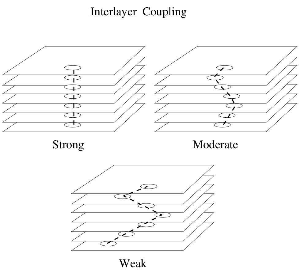
Figure 1: A single vortex line in an anisotropic superconducting material is
broken into a string of pancake vortices, one per layer. Here, the
magnetic field is applied normal to the plane of the layers. The coupling
between pancakes in different layers varies depending on the degree of
anisotropy in the material. Upper left: In a relatively isotropic material,
the pancakes are strongly coupled and the vortex line appears
as a rigid rod. Upper right: In materials with moderate anisotropy,
the vortex line is able to wander transverse to the direction of the
applied field. Lower center: In highly anisotropic materials, the coupling
between vortices becomes so weak that the individual pancakes may move
independently of each other within their respective layers, and
the elastic approximation breaks down.
An anisotropic superconductor can be modeled as
separate layers containing pancake vortices, where the magnetic field is
applied in a direction normal to the layers. Each magnetic flux line
is broken into pancake vortices, one per layer, with an attractive
inter-layer interaction between pancakes belonging to the same vortex.
(See Fig. 1).
For the form of the inter-layer
interaction, we choose a simple spring model.
For simplicity, we assume that the only inter-layer interactions are among
pancakes belonging to the same vortex, so that pancakes on different layers
belonging to different vortices do not interact.
The pancakes within a single layer, all of which belong to different
vortices, have a repulsive interaction.
This model, which does not employ the exact magnetic interactions
used in [20,21],
is similar to the model used in [19].
The overdamped equation of motion for vortex i in layer L is
fi,L = fivv + fivI + fivp = ηvi ,
(1)
where the total force fi,L on vortex i (due to the other vortices
in the same layer fivv, pancakes belonging to the same vortex in
adjacent layers fivI, and pinning sites in the same layer
fivp) is given by
fi,L
=
Nv ∑ j=1
f0K1
⎛ ⎝
|ri,L − rj,L |
λ
⎞ ⎠
^
r
ij,L
+
Np,L ∑ k=1
fp
ξp
|ri,L − rk,L(p)| Θ
⎛ ⎝
ξp − |ri,L − rk,L(p) |
λ
⎞ ⎠
^
r
ik,L
+
Aintf0 (|ri,L−ri,L−1|
^
r
iid
+ |ri,L−ri,L+1|
^
r
iiu
) .
Here, Θ is the Heaviside step function, K1 is a modified
Bessel function, λ is the penetration depth,
ri,L is the location of the ith vortex in layer L,
vi,L is the velocity of the ith vortex in layer L,
rk,L(p) is the location of the kth pinning site in layer L,
ξp is the pinning site radius, fp is the maximum pinning force,
Aint is the strength of the inter-layer interaction along a
single vortex line,
Np,L is the number of pinning
sites in layer L, Nv is the number of vortices, and
the force is measured in units of
f0 =
Φ02
8π2λ3
.
(2)
For a given layer L, the vortex-vortex unit vectors and
the vortex-pinning unit vectors are, respectively, given by
^
r
ij,L
=
ri,L−rj,L
|ri,L −rj,L|
,
^
r
ik,L
=
ri,L−rk,L(p)
|ri,L−r(p)k,L|
.
(3)
For a given vortex line i, the pancake vortex in layer L
is coupled to the following adjacent pancake vortices:
one in layer L−1, along ∧riid, (d for "down"), and
one in layer L+1, along ∧riiu, (u for "up").
These are given, respectively, by
^
r
iid
=
ri,L−ri,L−1
|ri,L−ri,L−1|
,
^
r
iiu
=
ri,L−ri,L+1
|ri,L−ri,L+1|
.
(4)
We take the pinning force to be fp = 0.55 f0, the
pinning density to be np = 4.0/λ2, and the
radius of the pinning sites to be ξp=0.12λ.
We consider either strong or moderate inter-layer interactions,
with Aint=2.0 or Aint=0.5, respectively.
Our sample is composed of N layers, where N ranges from 4
to 24. To handle the large number of pancake vortices in the sample,
we use a parallel molecular dynamics simulation. We divide the system
into regions, called domains, which are distributed among the
processors. Calculations for each region are carried out
simultaneously, and the processors remain coordinated by regular
communications using the Message Passing Interface [23]
protocol.
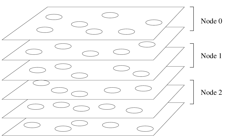
Figure 2: The one-dimensional domain decomposition used in parallelizing
the simulation.
The sample is broken into groups of layers. Here,
groups of two layers are shown. Each group is assigned to a node.
Each node communicates with the two nodes responsible for the
layers immediately above and below its domain. We use open boundary
conditions in the direction normal to the layers, so the two nodes
responsible for the top and bottom of the sample (nodes 0 and 2 in this
case) communicate with only one other node.
In our simulation, the domain decomposition is one-dimensional,
as shown in Fig. 2.
We break the sample into groups of layers, and assign each group to
a processor (referred to as "nodes" on the IBM SP2 machine).
Each node communicates with the two nodes containing the layers
immediately above and below its domain. We use open boundary
conditions in the direction normal to the layers, so the two nodes
responsible for the top and bottom of the sample communicate with
only one other node.
As the simulation runs, each node calculates the repulsive intra-layer
interactions of the vortices for every layer it contains. It then finds
the inter-layer interactions among the layers for which it is responsible.
The nodes then message-pass the positions of the vortices in their
end-most layers to the neighboring nodes, so that calculations of
interactions between layers on different nodes can be performed.
The straightforward one-dimensional domain decomposition that we use here is
ideal for this system. Since there are an equal number of vortices on each
layer, load balancing is automatically achieved, meaning that each
node must perform the same number of calculations for each molecular
dynamics time step, so no single node can get ahead or behind the
others. The only limitation on the number of
layers each node can contain is processor memory. On the IBM SP2
machine that we used, the processors could accommodate up to six layers each.
The overall number of layers in the sample is in principle limited only by
the number of nodes contained in the machine.
We typically used 8 nodes for the results presented here.
Figure 3: Schematic top view
(looking down on a single layer) of the sample geometry.
The sample region is the pinned area in the center of the figure, where
pins are represented by large open circles. At the edges of the sample
is an unpinned region. Vortices in this area simulate the externally
applied magnetic field. To construct a hysteresis loop, vortices are
gradually added to the unpinned region. The flux lines enter the sample
due to their own mutual repulsion and are trapped by pinning sites.
In order to generate magnetic hysteresis curves, we use a sample geometry
corresponding to a slab of anisotropic superconductor in a magnetic field
applied parallel to the slab surface [24].
The system is periodic in the plane
parallel to the applied field.
The actual sample region is heavily pinned, and extends from position
x=4 λ to x = 20 λ.
Outside the sample itself is a region with no pinning which extends from
x=0λ to x=4 λ and from x=20 λ to
x=24 λ (with 24 λ = 0λ according to our
periodic boundary conditions). A schematic diagram of the top view of
this sample geometry is shown in
Fig. 3.
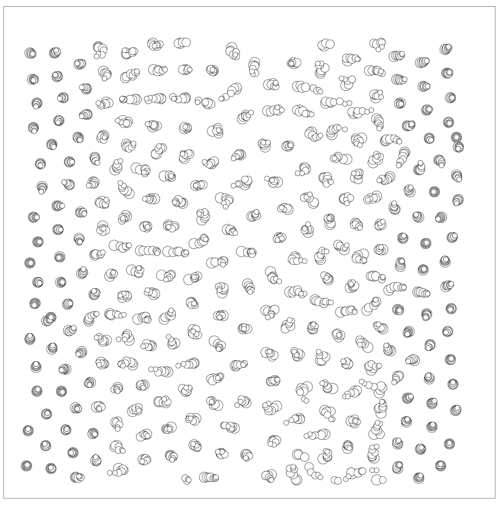
Figure 4: Vortex positions from a three-dimensional simulation. Circles of
a given radius indicate pancake vortices in a given layer, with the largest
circles falling in the lowest layer.
The external field region appears as an area of
evenly spaced vortices aligned with the magnetic field direction.
Inside the sample, the moderately coupled pancake vortices
bend as they interact with point pinning sites.
We simulate the ramping of an external field H by the slow addition of flux
lines to the outside unpinned region. Because there is no pinning in
this region, the flux lines attain a fairly uniform density,
and we may define the applied field H as Φ0 times this
density. Flux lines from the external region enter the sample
through points at the sample edge where the local energy is low. Thus,
our simulation models the real situation where vortices nucleate at such
low-energy regions at the surface.
An image of the vortices in our simulation is shown in Fig. 4.
Experimentally, what is typically measured is the average magnetization over
the sample volume. In our simulation, we calculate the average
magnetization
M=
1
4πV
⌠ ⌡
(H−B)dV ,
(5)
as a function of applied field for different pinning parameters.
Figure 5: Magnetization curves for a sample with 16 layers
containing columnar pins.
The same magnetization behavior is observed regardless of whether the
inter-layer vortex interaction is moderate
(Aint=0.5, large open diamonds)
or strong (Aint=2.0, small filled diamonds).
We first consider samples containing columnar pins, which are
modeled as a correlated line of parabolic traps, one in each layer
of the sample. If the magnetic field direction is aligned with the
columnar pins, then we expect the vortices to behave as perfectly rigid
rods. That is, the case of columnar pins can be accurately represented
by a two-dimensional simulation. We should therefore observe
behavior consistent with an effectively two dimensional system
[24]. As shown in Fig. 5 for
a sample containing 16 layers, we find
that the width of the hysteresis loop is not affected when the
inter-layer interaction force constant Aint is changed
from moderate coupling, Aint = 0.5, to strong coupling,
Aint = 2.0. This indicates that the three-dimensional character
of the vortex line does not play a role in the vortex-pin interactions.
Since columnar pins are able to pin a flux line along its entire length
without requiring the vortex to bend transverse to the field direction
[25],
allowing the vortex freedom to flex along its length does not change the
ability of a columnar pin to trap a vortex. Thus, in this case we
observe effectively two-dimensional behavior.
Figure 6: Magnetization curves for a sample with 16 layers containing randomly
located point pins.
Larger magnetization is observed when the inter-layer vortex interaction is
moderate (Aint=0.5, outer curve) than when it is
strong (Aint=2.0, inner curve), indicating that the
three-dimensional nature of the vortices is important in this case.
If the pinning sites in the sample are not correlated, but are instead
randomly scattered through the sample as point pins,
such as those created by proton irradiation [27],
then the three-dimensional
nature of the vortices becomes very important. We can see this in the
case of Fig. 6, where hysteresis curves from samples
with 16 layers containing random point pinning are shown. If the inter-layer
interaction is moderate, an individual vortex line is able to bend
significantly in order to take better advantage of the existing pinning
and be trapped by as many pinning sites as possible. When the
inter-layer interaction strength is increased and the flux lines become
correspondingly stiffer, individual vortices can no longer bend enough
to intersect a large number of pinning sites. The effective pinning
force on the stiff vortices is thus weaker than for the flexible vortices,
so the amount of hysteresis is reduced. This shows that the
character of the vortices in the third dimension cannot be neglected in
a sample containing point pinning.
Figure 7: Magnetization curves for two samples with 16 layers containing stiff
vortices (Aint=2.0) and an equal number of pinning sites.
In one sample, the point pins are arranged randomly, while in the
other sample, columnar pins are present.
The sample containing columnar pins produces a much larger magnetization.
In actual superconducting materials, point pins occur naturally due to
crystalline defects that form during production of the sample.
Columnar pins must be added artificially by irradiating the sample
with heavy ions [25,28]
or neutrons [26].
In experiments, it has been shown that the addition
of columnar defects significantly increases the width of the magnetization
curve, indicating that such irradiated samples have more desirable
vortex pinning characteristics. With our three-dimensional simulation,
we can compare the effects of point pins versus columnar pins on the
magnetization curve. In Fig. 7,
hysteresis curves for two samples with 16 layers and stiff vortices are
shown. Both samples contain the same number of pinning sites, but in
one sample the pins are spatially uncorrelated, while in the other
the pins are aligned into columns parallel with the applied magnetic
field. We see that the magnetization is significantly enhanced when
the pinning sites are columnar, in good agreement with experimental
results [28,29,30].
Figure 8: Magnetization curves for samples with 8 layers containing flexible
vortices (Aint=0.5) and columnar pinning sites. The columnar
pins are tilted with respect to the applied magnetic field by offsetting
each pin a distance α from the pin in the layer above. The offsets
used are: α = 0.0λ (filled circles), corresponding to a tilt
angle of 0 degrees, and
α = 0.10λ (filled triangles), corresponding to a tilt angle
of approximately 80 degrees.
The magnetization decreases when the field is tilted away from the direction
of the columnar pins.
Columnar pins are only effective at increasing the critical current
when the magnetic field is aligned with the columnar pins. As the
alignment is destroyed, the enhancement of pinning is reduced.
In Fig. 8, we show the results of
tilting the magnetic field direction with respect to the columnar pins
in a sample containing 8 layers and flexible vortices.
Rather than tilting the field lines in our simulation, we tilt the
columnar pins by displacing each pin a distance α
in a specified direction relative to the pin in the layer above.
As seen in Fig. 8,
tilting the field away from the pins results
in a loss of magnetization enhancement at low applied fields.
It is important to take into account the full three-dimensional nature
of vortices in anisotropic materials when studying the effects of
correlated pinning on the vortex behavior. If pinning sites are
regarded as point-like attractive centers scattered among the different
layers of the material, then changing the spatial correlation of these
sites can affect the vortex behavior.
Our model of vortices as spring-like chains of pancake vortices
reproduces expected experimental results:
Columnar pinning is more effective than point pinning, but
only when the field is aligned with the defects.
The effects of tilting the field are also in agreement with experiments.
The three-dimensional parallel simulation described here will be
useful in studying the dynamics of vortices interacting with a
wide array of samples.
If the model described here is extended to allow vortex cutting,
it will be possible to carry out careful studies of numerous topics
of current interest, including entangled vortex phases [31]
and flux transformer geometries [32].
Several extensions of these studies are possible.
For instance, it would be of interest to extend these studies
to superconducting samples with periodic arrays of columnar defects,
(e.g., [33]), which show commensurability effects in M(H).
These samples can reach much higher critical currents than
the ones with random arrays of pinning sites, and thus are
of potential technical importance.
We thank J. Clem, H. Marshall, and C. Reichhardt for helpful
discussions.
We acknowledge the hospitality of the Materials Science
Division of Argonne National Laboratory, and partial
support under DOE contract No. W-31-109-ENG-38.
FN acknowledges partial support from the
Center for the Study of Complex Systems and the Michigan
Center for Theoretical Physics at
The University of Michigan. This is preprint number MCTP-00-05.
CJO acknowledges support from the GSRP of the microgravity
division of NASA. Computing services were provided by
the Maui High Performance Computing Center, sponsored
in part by Grant No. F29601-93-2-0001, and by the
University of Michigan Center of Parallel Computing,
partially funded by NSF Grant No. CDA-92-14296.
J.R. Clem, Phys. Rev. B 43 (1991) 7837;
M. Benkraouda and J.R. Clem, Phys. Rev. B 53 (1996) 438;
A. Gurevich, M. Benkraouda, and J.R. Clem,
Phys. Rev. B 54 (1996) 13196;
J.R. Clem, T. Pe, and M. Benkraouda, Physica C 282-287 (1997) 311.
A. Tonomura et al.,
Nature 6717 (1999) 308;
C.H. Sow et al.,
Phys. Rev. Lett. 60 (1998) 2693;
N. Osakabe et al.,
Phys. Rev. Lett. 78 (1997) 1711;
J. Bonevich et al.,
Phys. Rev. B 57 (1998) 1200.
L. Civale, A.D. Marwick, M.W. McElfresh,
T.K. Worthington, A.P. Malozemoff, F.H. Holtzberg, J.R. Thompson,
and M.A. Kirk, Phys. Rev. Lett. 65 (1990) 1164;
L. Civale, M.W. McElfresh, A.D. Marwick, F. Holtzberg,
C. Feild, J.R. Thompson and D.K. Christen, Phys. Rev. B 43 (1991) 13732.
L. Civale, A.D. Marwick, T.K. Worthington, M.A. Kirk,
J.R. Thompson, L. Krusin-Elbaum, Y. Sun, J.R. Clem, and F. Holtzberg,
Phys. Rev. Lett. 67 (1991) 648.
D. Lopez, E.F. Righi, G. Nieva, F. de la Cruz, W.K. Kwok,
J.A. Fendrich, G.W. Crabtree, and L. Paulius, Phys. Rev. B 53 (1996) R8895;
D. Lopez, E.F. Righi, G. Nieva, and F. de la Cruz, Phys. Rev. Lett.
76 (1996) 4034.