Physical Review Letters 82, 3641 (1999)

Topological Invariants in Microscopic Transport on Rough Landscapes: Morphology, Hierarchical Structure, and Horton Analysis of Riverlike Networks of Vortices

A.P. Mehta, C. Reichhardt, C.J. Olson and Franco Nori

Department of Physics, The University of Michigan, Ann Arbor, Michigan 48109-1120

(Received 4 September 1998)

River basins as diverse as the Nile, the Amazon, and the Mississippi satisfy certain topological invariants known as Horton's Laws. Do these macroscopic (up to 103 km) laws extend to the micron scale? Through realistic simulations, we analyze the morphology and hierarchical properties of networks of vortex flow in flux-gradient-driven superconductors. We derive a phase diagram of the different network morphologies, including one in which Horton's laws of length and stream number are obeyed-even though these networks are about 109 times smaller than geophysical river basins.
Vortex River Basins
Simulation
Morphological Characterization
Horton Analysis
Concluding remarks
References

The nature of river basins[1,2,3,4], including their physical structure and evolution, has been a problem of major interest to civilized societies throughout history. Horton's laws are perhaps one of the most intriguing properties of river networks [1,2,3,4]. In order to apply them to a network, the individual streams composing the network must be identified and labeled with an order number, as in the top left corner of Fig. 1(a). The lowest order streams are the smallest outlying tributaries on the edges of the network, according to the Strahler ordering scheme. At each point where two tributary streams join, a new stream begins. Whenever two tributaries of the same order meet, the outgoing stream has an order number one higher than that of the tributaries. If two tributaries of different orders meet, the outgoing stream has the same order number as the higher ordered tributary. Eventually, all streams in the network combine to form the highest order (main) stream. The number of streams of order w is Nw, while Lw is the average length of streams of order w. Horton's laws state that the bifurcation ratio RB and the length ratio RL, given by RB = Nw / Nw+1 and RL = Lw+1/Lw, are constant, or independent of w. These ratios also provide the fractal dimension [1,2,3] of the rivers DFlogRB/logRL. Geophysical river basins [1,2,3] typically have values of RB ≈ 4 and RL ≈ 2. Do these (Horton's) laws apply to microscopic landscapes? Here we present evidence that these macroscopic laws are obeyed at the microscopic scale by river-like networks of flowing quantized magnetic flux.
Vortex River Basins.- Near the depinning transition, magnetic vortices in type-II superconductors move in intricate flow patterns that have been seen both in computer simulations and in experiments, including finger-like or dendritic shapes as well as the filamentary flow of vortices in river-like paths and networks (see, e.g., [5,6,7] and references therein). Despite the ubiquity of the river-like pathways produced by the vortex motion, very little work has been done towards characterizing the morphology of these flow patterns. Moreover, concepts and ideas used for decades to characterize geophysical river basins have not been applied to the study of the microscopic flow through tree-shaped channel networks. This is surprising since the underlying physics of vortex and geological rivers offers striking similarities: driven non-equilibrium dissipative systems displaying branched (or ramified) transport among metastable states on a rough landscape [8]. One is driven by the Lorentz force and the other by gravity. Like geophysical rivers, vortex flow basins exhibit sinuosity (i.e., tortuosity), anabranching, braiding, occasional sudden floods, and other features that make them remarkably similar to geophysical rivers [1]. Indeed, some satellite photographs of river basins are strikingly similar to the channels produced by vortex motion. However, significant differences also exist, including: flow direction, quantized flux flow versus continuum water flow, compressible vortex lattice versus incompressible fluid, negligible inertia with overdamped vortex dynamics versus massive fluid, non-erosional versus erosional landscape, peripheral flux sources versus uniform rain, and correlated long-range versus short-range interactions (so the rapidly varying vortex-vortex repulsion landscape smoothes out the underlying static pinscape). This strongly-correlated vortex dynamics generates flux motion that can be either continuous-flow type, like water, or intermittent stick-slip-type motion-depending on the balance of forces. Also, vortices typically move over relatively flat landscapes with many divots, as opposed to the mountain-range-like very rough landscapes of some geophysical rivers. Moreover, vortex river basins occur inside materials at approximate scales between 1 to 100 μm, much smaller than geophysical river basins (of up to 103 km)-and also spanning a smaller range of length scales. Thus, given these numerous similarities and differences, it is very unclear a priori which macroscopic results carry over to the microscopic domain.
By conducting realistic simulations of slowly driven vortices moving over many samples, we have identified several distinct network phases. These vortex basins appear in the initial penetrating front of vortices[6,7]. Remarkably, we find that: for a wide range of parameters networks of vortex channels obey Horton's laws just as geophysical river networks do. This is remarkable, given the many physical differences between basins of flux quanta and geophysical rivers and that they move over very different types of potential-energy landscapes. Unlike previous work, here we first present a detailed list of analogies and differences between river basins and networks of vortex channels. Afterwards, we present the first morphological phase diagram for vortex motion. Finally, we analyze the hierarchical structure of the vortex channels.
Fig1.png
Figure 1: Snapshots of northbound vortex pathways: (a) Hortonian (when the pinning force, fp  , is stronger than the vortex-vortex repulsion fvv  ; i.e., at low B and high fp); (b) braided (when fp is comparable to fvv  : B ≈ 3 Bϕ / 2 [7]); and (c) dense (when fp << fvv  ; i.e., for B > 2 Bϕ; or at any field for low fp). Here, np=0.75/λ2. The matching field Bϕ occurs when the number of vortices Nv equals the number of pinning sites Np. Bϕ is used to quantify the relative strength of pinning versus vortex-vortex repulsion [7].
Simulation.- We model a transverse 2D slice (in the x-y plane) of an infinite zero-field-cooled T=0 superconducting slab containing flux-gradient-driven 3D rigid vortices that are parallel to the sample edge [6,7]. Vortices are added at the surface at periodic time intervals, and enter the superconducting slab under the force of their own mutual repulsion [6,7]. The slab is 36λ×36λ in size, where λ is the penetration depth. The vortex-vortex repulsive interaction is correctly modeled by a modified Bessel function, K1(r/λ). The vortices also interact with 972 non-overlapping attractive parabolic wells of radius ξp=0.3λ. The density of pins np is np=0.75/λ2. All pins in a given sample have the same maximum pinning force fp, which ranged from fp=0.3f0 to fp=6.0f0 in thirteen different samples. For each sample type, we considered five realizations of disorder. Thus, the five points at each pinning force, delineating the broad crossover boundary between Hortonian and braided phases in Fig. 2, refer to these five realizations of disorder. A sixth point, indicating the average value from the five trials, is not visible when it overlaps with another point. We measure all forces in units of f002/8π2λ3, magnetic fields in units of Φ02, and lengths in units of the penetration depth λ. Here, Φ0 is the flux quantum.
The overdamped equation of vortex motion is fi = fivv + fivp = ηvi, where the total force fi on vortex i (due to other vortices fivv, and pinning sites fivp) is given by fi = ∑j=1Nvf0  K1(|rirj|/λ)rij + ∑k=1Np(fpp)|rirk(p)|  Θ[ ξp − |rirk(p)| ]rik  . Here, Θ is the Heaviside step function, ri (vi) is the location (velocity) of the ith vortex, rk(p) is the location of the kth pinning site, ξp is the pinning site radius, Np (Nv) is the number of pinning sites (vortices), rij = (rirj)/|rirj|, rik = (rirk(p))/|rirk(p)|, and we take η = 1.
Fig2.png
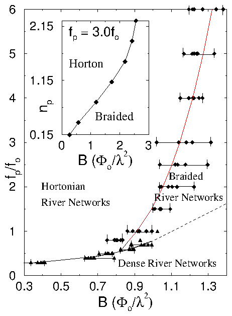
Figure 2: The vortex river network morphological phase diagram for pinning force, fp, versus magnetic field, B, for np=0.75/λ2 (thus, here Bϕ = 0.75  Φ0 / λ2). In regions of very low pinning force, dense vortex river networks dominate. For higher pinning fp's, the Hortonian rivers become braided when B grows. For samples with significant amount of pinning, it is the initial front (with low local density of field lines B, B < 3 Bϕ / 2 [7], and thus dominant pinning force fp) which branches out in a Hortonian manner. Behind this initial front follows the (intermediate-B) braided region. Further behind, follows the (large-B) dense-flux regime. The inset shows the shift in the Horton-braided boundary fp=3.0f0 as the pinning density, np, is changed. As np is increased, the Horton-braided boundary shifts towards higher B. The broad crossover boundaries are in the region of triangles and rhombuses. The (power-law-fit) lines are just guides to the eye. The dense-braided crossover at high-fields (dashed) is an extrapolation of the power-law-fit for low fields; the former is very difficult to compute because it requires a large number of vortices monitored over very long times.
Morphological Characterization.- In order to identify and characterize the vortex river networks formed as the flux-gradient-driven front initially penetrates the sample, we divide our simulation area into a 300 ×300 grid. Each time a vortex enters a grid element, the counter associated with that element is incremented. All grid elements that are visited at least once by a vortex are considered part of the network [6]. The maximum number of vortices in the sample is approximately 1200. The pinning density np and radius ξp were kept constant at np = 0.75/λ2 and ξp=0.3λ, while the pinning force fp varied from sample to sample. We also performed additional simulations in which fp was kept constant and np varied from np=0.15/λ2 to np=2.15/λ2.
We observed three distinct vortex river network morphologies, depending on the local magnetic field B and the pinning force fp, as indicated in one of our main results: the "morphological phase diagram" in Fig. 2. In Fig. 1 the vortex trajectories are presented for the three morphologies. In samples with low pinning force values, fp <~0.75f0 (see Fig. 2), vortices flow throughout the sample, producing dense vortex river basins. These become space-filling for large times-or large fields since the external field is slowly ramped up. An example of the vortex channels in this regime, as they appear after 160000 MD steps, is shown in Fig. 1(c). If the simulation is allowed to proceed for a larger number of MD steps, the channels eventually fill the entire region shown in Fig. 1(c). For stronger pinning, fp >~1.0 f0, and low vortex densities B <~ Φ02 ≈ 3 Bϕ/ 2, we observe branched "Hortonian" river networks that follow Horton's laws of stream number and length [see Fig. 1(a)]. At higher magnetic fields B >~Φ02 ≈ 3 Bϕ/2 , the vortex rivers become highly braided or interconnected and are no longer Hortonian in morphology [see Fig. 1(b)]. Unlike the dense networks of Fig 1(c), where preferred vortex paths are uncommon, in the braided regime vortices consistently move along certain pathways, while in some areas of the sample vortex motion rarely occurs.
Fig3.png
Figure 3: (a) Fraction Rups of unoccupied pinning sites (ups) versus B for six samples with different fp's. We find a change in the rate at which pins become occupied with increasing field: it decreases noticeably for B > Bϕ. (b) The length ratio RL and DF/dc=logRB/logRL, versus the pinning force, fp. The stream dimension, dc, is one. Only the trend in the fractal dimension DF can be observed from above because the error bars for RL and DF/dc are ±0.1. The lines are power-law best fit curves, which only provide a guide to the eye. The formula for DF gives values slightly above 2, because it assumes that Horton's laws hold at all length scales, while our vortex basins only span a very limited range of length scales.
For low pinning forces in the dense network regime, vortex motion occurs both interstitially (with the vortices moving only in the areas between pinning sites) and by means of depinning. If vortex depinning is occurring in a landscape with traps of comparable strength, no favored paths for flux motion can form, leading to the observed dense pathways. The Hortonian and braided regimes arise once the pinning is strong enough that predominantly interstitial motion occurs. That is, pinned vortices almost never depin. Other vortices are prevented from moving close to a pinned vortex by the vortex-vortex repulsion, which has a longer (by near two orders of magnitude) range than the attraction of each pinning site. Since there are regions of the sample (i.e., at or near pinned vortices) where flux motion does not occur, the flow of the moving vortices must be concentrated in certain well-defined regions or rivers, leading to the formation of either Hortonian or braided rivers.
The broad crossover between Hortonian and braided rivers occurs when the flux density has increased enough that a large fraction of the pinning sites are occupied. In Fig. 2, the crossover region increases from B ≈ 0.9 Φ02 for fp = 1.0f0, to B ≈ 1.3 Φ02 for fp = 6.0f0. In each case, the crossover occurs at vortex densities higher (3 Bϕ / 2 <~B < 2 Bϕ) than the matching field Bϕ=0.75 Φ02, when Np=Nv [11]. This is in agreement with the results for the inset of Fig. 2, which shows that the transition from Hortonian rivers to braided rivers occurs at higher vortex densities as np (and thereby the matching field) is increased. Additional support for this interpretation comes from examining the fraction Rups of unoccupied pinning sites [Fig. 3(a)]. At the matching field, Bϕ=0.75  Φ02, only about 65% of the pins are occupied [7,11]. The pins are not fully occupied until a field of B ≈ 1.4  Φ02 ≈ 2  Bϕ is applied-when the potential energy landscape experienced by the moving vortices becomes much more uniform.
Fig4.png
Figure 4: The number of streams Nw of order w, and their lenghts Lw, for vortex river networks with three different pinning forces fp. Six different fp's gave virtually identical plots-all obeying Horton's laws.
Horton Analysis.- In order to determine whether the vortex river networks we observe obey Horton's laws, we performed Hortonian analysis on five different realizations of disorder for each of eight different pinning forces fp falling within the Hortonian regime. In each trial, a branching river was identified for analysis. The numbers Nw and lengths Lw of streams of order w = 1 to 4 were recorded. [9] Representative plots of the type used to determine the length ratio, RL=Lw+1/Lw, and the bifurcation ratio, RB=Nw/Nw+1, are shown in Fig. 4. In the best fit exponential regressions used to extract RL and RB, the average correlation coefficient was  0.99, indicating a good fit to the Hortonian relationships. The average values for RB and RL throughout the Hortonian river region were RB = 3.99 ±0.18 and RL = 2.04 ±0.12, in excellent agreement with geophysical rivers. [1,10].
The characteristics of the Hortonian river networks are dependent on the pinning force fp. In Fig. 3(b) we plot the length ratios RL, and fractal dimensions DF, for each pinning force in the Hortonian region. The braching ratio (not shown) is roughly constant as fp is varied. Changing the pinning force alters the ease with which individual vortices can be depinned, and thereby changes RL and Df/dc. As the pinning force decreases, it is more likely that some vortices will be depined and form new pathways of vortex motion. This will decrease the length of the higher order rivers by cutting short how far the vortex channels propagate before bifurcating. Therefore RL will decrease with decreasing fp. Since a larger number of paths are created the Df will increase with decreasing fp, in agreement with Fig. 3(b).
Concluding remarks.- We have analyzed the morphologies of flux-flow channels slowly driven to its marginally stable state, as a function of flux density and disorder strength. We have identified three distinct morphologies[12] which include: a (large B) dense network regime, where flow can occur anywhere; a braided network regime, where flow is restricted to certain regions; and a (low B) Hortonian network regime, where Horton's laws of length and branching ratio are obeyed in agreement with geophysical rivers. Indeed, it seems promising to analyze tree-shaped channel flow at the microscopic level adapting concepts that have already been successful in treating macroscopic river basins. These types of analysis are largely unexplored. The direction and success of such an approach constitutes an open and fascinating area.
CJO (APM) acknowledges support from the GSRP of the microgravity division of NASA (NSF-REU). We thank the Maui Supercomputer Center, R. Riolo, and the UM-PSCS for providing computing resources. We thank F. Marchesoni, M. Bretz, E. Somfai, D. Tarboton, and S. Peckham for their comments.
[1]
I. Rodriguez-Iturbe and A. Rinaldo Fractal River Basins: Chance and Self-Organization (Cambridge, NY, 1997).
[2]
G. Korvin, Fractal Models in the Earth Sciences (Elsevier, Amsterdam, 1992); D.L. Turcotte, Fractals and Chaos in Geology and Geophysics (Cambridge, Cambridge, 1992); J. Feder, Fractals (Plenum, New York, 1988); B.B. Mandelbrot, The Fractal Geometry of Nature (Freeman, San Francisco, 1983).
[3]
R.E. Horton, Bull. Geol. Soc. Am. 56, 275 (1945); D.G. Tarboton, R.L. Bras, and I. Rodriguez-Iturbe, Water Resour. Res. 24, 1317 (1988); 25, 2037 (1989); 26, 2243 (1990); S.D. Peckham, ibid 31, 1023 (1995); D.G. Tarboton, J. Hydr. 187, 105 (1996); J.G. Masek and D.L. Turcotte, Geology, 22, 380 (1994); I. Yekuteli, B.B. Mandelbrot, J. Phys. A, 27, 285 (1994).
[4]
E. Somfai and L.M. Sander, Phys. Rev. E 56, R5 (1997); S. Kramer and M. Marder, Phys. Rev. Lett. 68, 205 (1992); A. Rinaldo et al. ibid. , 70, 822 (1993); J. Watson and D.S. Fisher, Phys. Rev. B 55, 14909 (1997).
[5]
F. Nori, Science 278, 1373 (1996); T. Matsuda, ibid. 1393 (1996); H.J. Jensen, et al. Phys. Rev. B 38, 9235 (1988).
[6]
C.J. Olson, C. Reichhardt, and F. Nori, Phys. Rev. Lett. 80, 2197 (1998).
[7]
C. Reichhardt et al. Phys. Rev. B 53, R8898 (1996).
[8]
Recent efforts have been made to link river basins to self-organized-criticality [1]. Indeed, when Np > Nv (the Hortonian regime in Fig. 2), the adiabatic dynamics of vortices also exhibits avalanches with power-law size distributions [C.J. Olson, C. Reichhardt, and F. Nori, Phys. Rev. B 56, 16108 (1997)].
[9]
Streams of order w=5 and above were very rare in our samples because our landscapes are flat, with small parabolic potential wells on it. Thus, the vortex microscopic landscape is very different from the quite rough mountain-like landscapes used to model some geophysical river basins. Therefore, Horton's laws for vortices do not extend over a wide range of length scales.
[10]
The random topological model, among others, suggest that many networks fit Horton's laws. However, these models ignore the fundamentally important role of the third dimension: the landscape elevation. Also, these models ignore the physical laws that describe the carving of individual channels. For macroscopic river basins, the role of both chance and necessity for Horton's laws have been very lucidly discussed in [1]. Also, it is unclear how these arguments can be extended to the microscopic scale because the motion of flux quanta is highly-correlated. For instance, one vortex can interact with a very large number of other quanta within a large radius, given by λ. This type of collective correlated motion is absent from the simple random topological network models. Also, the lack of "uniform rain" and erosion inside materials, common in river basin models, makes it difficult to make comparisons with previous work on river basins. Moreover, there is no consensus on the precise conditions required to obtain Horton's laws at the macroscopic level (let alone at the microscopic quantum regime). These issues are beyond the scope of this paper and will be explored elsewhere.
[11]
This is due to the fact that a fraction of pinning sites remains unoccupied at the matching field, as shown in experiments and simulations [7]. This is a consequence of the random spatial distribution of the pinning. If one pinning site is very close to a second site containing a vortex, the repulsive force of the trapped vortex will prevent the empty pin from being occupied until the vortex density increases further.
[12]
Videos with examples of vortex river networks appear in http://www-personal.engin.umich.edu/~nori


File translated from TEX by TTHgold, version 4.00.

Back to Home