Physical Review B 52, 10441 (1995)

Microscopic Derivation of Magnetic Flux Density Profiles, Magnetization Hysteresis Loops, and Critical Currents in Strongly Pinned Superconductors

C. Reichhardt, C. J. Olson, J. Groth, Stuart Field, and Franco Nori
Department of Physics, The University of Michigan, Ann Arbor, Michigan 48109-1120

(Received 18 May 1995)

We present a microscopic derivation, without electrodynamical assumptions, of B(x,y,H(t)), M(H(t)), and Jc(H(t)), in agreement with experiments on strongly pinned superconductors, for a range of values of the density and strength of the pinning sites. We numerically solve the overdamped equations of motion of these flux-gradient-driven vortices which can be temporarily trapped at pinning centers. The field is increased (decreased) by the addition (removal) of flux lines at the sample boundary, and complete hysteresis loops can be achieved by using flux lines with opposite orientation. The pinning force per unit volume we obtain for strongly-pinned vortices, Jc B  ∼ np fp1.6, interpolates between the following two extreme situations: very strongly-pinned independent vortices, where Jc B  ∼ np fp, and the 2D Larkin-Ovchinikov collective-pinning theory for weakly-pinned straight vortices, where Jc B  ∼ np fp2. Here, np and fp are the density and maximum force of the pinning sites.
I. INTRODUCTION
II. SIMULATION
A. Sample geometry and time-dependent field
B. Equations of motion
III. MAGNETIC-FLUX-DENSITY PROFILES
IV. MAGNETIZATION HYSTERESIS LOOPS
V. CRITICAL CURRENT VERSUS PINNING DENSITY AND STRENGTH
VI. CONCLUSIONS
References

I.  INTRODUCTION

Flux distributions in type-II superconductors are commonly inferred from magnetization and critical current measurements[1] and interpreted in the context of the Bean model[2] or its variations. The Bean model, which has been widely used for over three decades, postulates that the current density in a hard superconductor (i.e., with strong pinning) can only have three values: −Jc, 0, and +Jc, where Jc is the critical current density, which is independent of the local magnetic flux density B(x,y,t). The Bean model and its many variants make no specific claims with regard to the microscopic mechanism controlling the trapping of vortices. Bean's postulate, Jc=constant, was modified several times by Kim et al.[3]: Jc  ∼ 1/ B   [3a]; Jc  ∼ 1/(b0+B)   [3b,3c]; Jc  ∼ 1/(b0+B+b2B2+b3B3+…)   [3b]; where bi are constants. On the other hand, Fietz et al. [4] suggested that Jc  ∼ exp(−B/b0)  ; while Yasuk¯ochi et al. [5] suggested Jc  ∼ 1/B1/2. These, and other proposals made during the 1960s, were followed by several other phenomenological modifications of Jc(H) during the following two decades[1,6]. A microscopic description, without assuming any particular B-dependence of Jc, of these flux distributions-in terms of interacting vortices and pinning sites-can be very valuable for a better understanding of commonly measured bulk quantities.
One of the most effective methods of investigating the microscopic behaviour of flux in a hard superconductor is with computer simulations (see, e.g., [7,8], and references therein). In this paper, we present molecular dynamics (MD) simulations of the evolution of rigid flux lines in a hard superconductor. We first introduce our model for vortex-vortex and vortex-pin interactions as well as the corresponding antivortex interactions. We then investigate the flux profile which results from a varying applied field; from such flux profiles we obtain full hysteresis loops indicating that our model has the essential microscopic ingredients underlying the experimentally measured macroscopic quantities. We also investigate the behaviour of Jc(H) for a controlled range of pinning parameters.

II.  SIMULATION

Our simulation geometry is that of an infinite slab of superconductor in a magnetic field applied parallel to the slab surface. Thus, demagnetization effects are unimportant. We also treat the vortices as perfectly stiff, so that we need to model only a two-dimensional (2D) slice of the 3D slab. Our system is periodic in the plane perpendicular to the applied field, and we measure distances in units of the penetration length λ. Here, we present results for a system of size 36λ×36λ. The simulation, described in further detail below, consists of slowly ramping an external magnetic field. Flux lines enter the edge of the sample and their positions are allowed to evolve according to a T=0 MD algorithm. The resulting vortex distributions at any external field can then be deduced as a function of distance into the sample.
Fig1.png
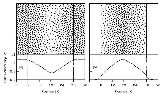
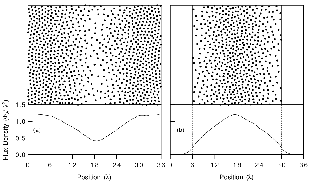
Figure 1: Top view of the region where flux lines, indicated by dots, move. (a) Snapshot during the initial ramp-up phase, (b) snapshot of the remnant magnetization after ramping down the external field. The bottom panels show B(x) = (36 λ)−1036λ dy  B(x,y), i.e., the flux density profile versus x, averaged over the vertical direction y. The 24 λ×36 λ sample has 3456 pinning sites, and fp=0.9f0.

A.  Sample geometry and time-dependent field

The actual sample region is heavily pinned, and extends from position x=6λ to x=30 λ (Fig. 1). Outside the sample itself is a region with no pinning which extends from x = 0 λ to x=6 λ and from x = 30 λ to x=36 λ (with 36λ = 0λ according to our periodic boundary conditions).  This sample geometry is shown in the upper panels of Fig. 1. Here, the sample (pinned) region occupies the central 2/3 of the system, and the unpinned region the outer 1/3.
We simulate the ramping of an external field by the slow addition of flux lines to the outside unpinned region. Because there is no pinning in this region, the flux lines there will attain a fairly uniform density, and we may define the applied field H as Φ0 times this density. Flux lines from the external region will move into the sample through points at the sample edge where the local energy-as determined by the local pinning and vortex interaction-is low. Thus, our simulation models the real situation where vortices nucleate at such low-energy regions at the surface.
Further, in a real superconductor, vortices near the surface are not expelled by their interior neighbors because of a field-induced Meissner current flowing at the surface. Again, our external "bath" of vortices simulates this behavior by providing a balancing inward force, proportional to the external field, on those vortices near the sample boundary.

B.  Equations of motion

The force per unit length [1] between two vortices located at ri and rj is
 fvv = Φ02

8 π2 λ3
 K1
| rirj |

λ

 .  
(1)
We model the vortex-vortex force interaction in its exact form by using the modified Bessel function K1. This force decreases exponentially at distances larger than λ, and we cut off the (by then negligible) force at distances greater than 6λ. Further, we have cut off the logarithmic divergence of the force for distances less than 0.1λ. These cutoffs were found to produce negligible effects on the dynamics for the range of parameters investigated. Thus, the force (per unit length) on vortex i due to other vortices (ignoring cutoffs) is  fivv =  ∑j=1Nv  fv  K1(|rirj| / λ)  rij  . Here, the rj are the positions of the Nv vortices within a radius 6λ,  rij = (rirj) / |rirj| ,  fv = ±f0, and
 f0 = Φ02

8 π2 λ3
 .
(2)
The sign of the interaction is determined by fv ; we take fv = +f0 for repulsive vortex-vortex interactions and fv = −f0 for attractive vortex-antivortex interactions. A vortex and antivortex annihilate and are removed from the system if they come within 0.3 λ of one another [1]. Forces are measured in units of f0, lengths in units of λ, and fields in units of Φ02.
We model the pinning potential[9] as Np short-range parabolic wells at positions rk(p). The equation of motion for a vortex moving with velocity v is fv, where η is the viscosity ( ≈ Φ0 Hc2n, with ρn being the normal-state resistivity). Thus, the overall equation for the overdamped motion of a vortex subject to vortex-vortex and pinning forces is
 fi = fivv + fivp = ηvi  ,
(3)
where
fi
=
  Nv

j=1 
 fv  K1
|rirj|

λ

 
^
r
 

ij 
+
Np

k=1 
fp

ξp
 |rirk(p)|  Θ
ξp − | rirk(p) |

λ

 
^
r
 

ik 
 .
(4)
Here, Θ is the Heaviside step function, ξp is the range of the pinning potential, and fp is the strength (maximum pinning force) of each well, measured in units of f0. For all the simulations presented here ξp = 0.12λ and η = 1. The parameters we vary here are the pinning strength fp and the average distance between pinning sites dp (which determines the pinning density np via np=1/dp2). Many other parameters can be varied, making the systematic study of this problem very complex. A more thorough investigation with different pinning-potential ranges, pinning potential-shapes, non-uniform strength distributions, and non-random pinning positions will be presented elsewhere. Here, the pinning sites have uniform strengths and are placed in the sample at random, but non-overlapping, positions. The pinning strength fp is varied from 0.2 f0 to 1.0 f0, and dp is varied from λ/3 to λ  (i.e., the pin density np varies from 1/λ2 to 9/λ2).

III.  MAGNETIC-FLUX-DENSITY PROFILES

Several general features of our simulations are shown in Fig. 1. In the upper frame of Fig. 1a, we show a top view of the vortex positions after the external field has been ramped up from zero. As we have stated, this external field is represented by the vortices in the unpinned regions to the left and right of the central, pinned, sample region. Here, vortices have been added to the unpinned region to a final density of about 1.2 vortices/λ2; since each vortex carries a flux Φ0, this corresponds to a magnetic field of 1.2  Φ02. For a real superconductor with a penetration depth of, e.g., 1000Å , this corresponds to H=2.5 kOe.
We note in Fig. 1(a) that many of the vortices added to the unpinned region have been forced into the central sample region at this stage. They do not do so uniformly due to the presence of 3456 pinning sites (not shown), with a typical intersite distance of λ/2 and fp=0.9 f0. We see the characteristic density gradient determined by a balancing of the vortex-vortex forces with the local pinning forces. Since this gradient was achieved in our simulation solely by the slow ramping of an external magnetic field, we have obtained the field profiles inside a pinned superconductor using only microscopic information such as vortex-vortex and vortex-pin interactions. We should also contrast our simulations with those modeling current-driven vortices. In such simulations the driving force on each vortex is somewhat artificially modeled by an externally-imposed "uniform" current. Our simulation correctly models the driving force as a result of local interactions.
The lower frame of Fig. 1a shows the resulting flux density profiles, found by averaging the vortex density over slices parallel to the sample edges. Such profiles clearly show the essentially constant flux density in the external regions, and the detailed nature of the flux gradient within the sample. Of course, these profiles may be obtained at any value of the external field. Figure 1b shows the system after the external field has been ramped down from a high value to zero. The small field outside the sample is an artifact due to the smearing of the vortex fields. Now, flux remains trapped within the sample and the field gradient has changed sign. We notice that near the sample edges, where the field is small, the gradient in the flux density is quite large. Thus our simulation correctly models the increase in flux gradient (or, equivalently, critical current) at low fields, where intervortex interactions are weak and pinning dominates.
beanFig2.png
Figure 2: Magnetic flux density profiles B(x) for the (1) initial ramp-up phase, (2) ramp-down stage reaching a negative field, and (3) final ramp-up phase, for the same sample described in Fig. 1 and the text. The flat plateaus on either side of the sample show the density in the unpinned region, mimicking the external field, and the jagged ∨- and ∧-shaped profiles correspond to the flux density in the pinned region.
In Fig. 2 we show flux density profiles for a complete cycle of the field, with the same sample parameters as in Fig. 1. During the initial ramp-up stage (Fig. 2, left), we increase the external field from zero to a final value of about 1.9 Φ02. We see the evolution of the internal flux profile from first penetration at low fields, to the first complete penetration at a field H* ≈ 0.8 Φ02, to higher values of B at larger H. We again note the flux gradient is quite high at low fields, but becomes flatter-and less field-dependent-at high fields.
Of course, in real superconductors no vortices will enter the sample until H > Hc1 ≈ (lnκ/ 4 π) (Φ02) , where κ = λ/ξ. However, for κ's in the wide physically relevant range from 2 to 100, Hc1 varies from 0.05   Φ02 to 0.36   Φ02. Thus, Hc1 is small in the range of fields we explore. In any event, since we are only interested in the mixed state and not the Meissner phase, we will work in the approximation where Hc1 is negligible.
During the ramp-down stage (Fig. 2, center), the field is lowered through zero to large negative values. The ramping down is initially effected by simply removing vortices from the unpinned region. However, after the external field reaches zero, it is reversed by the addition of antivortices in the unpinned region. During the beginning of this ramp-down stage, we note the appearance of the characteristic "gull-wing" flux profile as the internal remnant flux located close to the sample edges begins to be removed. Notice that at external fields near zero the internal field hardly changes at all as the external field is swept. This is again because of the very steep gradients possible near zero field, where pinning dominates. Thus, the effect of a change in an external field near zero propagates only a very small distance into the sample.
As the field decreases below H=0 (in Fig. 2, center), B(x) continues to have its ∧-shaped profile. We note that for small negative fields the sample contains both vortices and antivortices. However, the pinning for both types is attractive, and so they remain locally trapped and annihilate only when their mutual attraction overcomes the pinning. This only occurs when they are closely spaced, within 0.3 λ. Finally, in the last ramp-up stage (Fig. 2, right), the full cycle is completed by increasing the field from the large negative value up to a large positive field, where the flux profile looks identical to the initial ramp-up stage of the cycle.
One clear advantage of our simulation is that we can obtain direct spatio-temporal information on the distribution of flux inside the sample. However, experimentally this is quite difficult, especially for bulk samples. Instead, average quantities, like magnetization curves, are typically obtained. From the field cycles shown in Fig. 2, we can easily obtain such magnetization loops from our simulation. Further, in our simulation it is simple to vary microscopic parameters such as pin density and strength. Thus, our simulations allow for a systematic study of the dependence of macroscopic measurements, such as the magnetization, on microscopic system parameters. It may also be possible to use our results in the reverse problem, so that some understanding of the microscopics of the pinning [9] may be obtained from experimentally determined macroscopic measurements.
Fig3.png
Figure 3: Magnetization hysteresis curves M(H(t)). In (a) the maximum pinning force is varied (fp=0.9f0, 0.55f0, 0.2f0) for a fixed average distance between randomly distributed pinning sites, dp=λ/2 (i.e., λ2 np=4).  In (b) the pinning-site density np is varied while fp=0.55 f0. A higher value of fp and/or np increase Jc ( ∼  width of the M(H) hysteresis loop) in the manner shown in Fig. 4. For each M(H) loop shown, the maximum number of flux lines inside the pinned sample is about 1000.
Color figure

IV.  MAGNETIZATION HYSTERESIS LOOPS

Experimentally, what is typically measured is the average magnetization over the sample volume. In our simulation, we thus calculate the average magnetization

M
 
= 1

4 πV

(HB)  dV  .
(5)
In Fig. 3 we construct magnetization loops as two key sample microscopic parameters-the pinning density and strength-are varied. Fig. 3a shows complete magnetization loops obtained with the density of pins held constant at 4/λ2, but at three different values of the pinning strength fp. One can see clearly that by increasing the pinning strength the hysteresis loops become much wider. This is because a large pinning force yields a large field gradient. Thus M, which is essentially the difference between the internal and external fields, will be larger for large fp. For instance, the remnant M is larger for stronger pinning. The M(H) loops all show a maximum when the external field is small (HH*) and close to H*. This again is due to the pinning being most effective for low fields (HH*). Figure 3b shows magnetization loops obtained for several pinning densities. Experimentally, one may systematically vary this parameter by the introduction of columnar defects using irradiation [1,10].

V.  CRITICAL CURRENT VERSUS PINNING DENSITY AND STRENGTH

Although magnetization loops are very useful for comparison with experimental data, we have emphasized that our simulations allow us to directly compute the local flux distribution inside the sample. Thus, we may directly measure the local critical current density Jc using Maxwell's equation dB/dx = μ0 J. At every point on flux density profiles such as Fig. 2 we may compute the local slope ( = dB/dx) and the corresponding local field B. This allows us to determine a large number of values of Jc(B). We then bin these values to obtain suitably averaged curves of Jc vs. B.
As we have discussed, there are in the literature a great variety of functional dependences of Jc on B, corresponding to different ad hoc electrodynamical assumptions. The original Bean model predicts Jc to be independent of B. The varying slopes of the flux density in Fig. 2 show that this prediction is not borne out in our simulation (except at relatively high-fields where the vortex-vortex force dominates; e.g., for weak-pinning samples with λ2 np = 4.0, fp=0.2f0). Kim et al.[3] have proposed that the critical current depends on B as
α = Jc (B + b0)  ,
(6)
where α is field-independent and has units of force per unit volume. In this model, plots of 1/Jc vs. B should appear as straight lines with slopes 1/α and intercept b0/α. The physical interpretation of the constant b0 in Kim's model is unclear[3].
Fig4.png
Figure 4: (a) 1/Jc(B) for several values of the pin density np (and fixed pinning-site strength fp); (b) 1/Jc(B) for several values of fp (and fixed np). The insets show the dependence of the maximum pinning force α on fp (dark triangles) and on np (open circles) The values of α are obtained from the (solid line) linear fits shown in the larger panels.
In Fig. 4 we plot 1/Jc vs. B, with Jc determined from our flux density plots during the initial ramp up phase. We plot 1/Jc for several realizations of the pinning density np and strength fp. Fig. 4a shows 1/Jc vs B for four different field sweeps with the pinning density varied from 1.0/λ2 to 9.0/λ2; in Fig. 4b we vary the pinning strength from 0.2 f0 to 0.9 f0. Over a large region of the field, we find that 1/Jc is indeed linear in field, as in Kim's model. We can then fit the linear portions of each curve to straight lines as shown, and extract the inverse slope α. For fields such that B >> b0, Kim's relation reads α ≈ Jc B which is the Lorentz force per unit volume. Since this force is exactly balanced by the pinning force, we can interpret α as the maximum pinning force per unit volume. b0 is typically in the range of 0.4 to 0.7 Φ02, but even below b0, α is clearly a measure of the relative effectiveness of the pinning.
In the inset to Fig. 4a, we plot the values of α determined from the slopes of the 1/Jc curves as a function of the pinning strength fp or density np. The pinning force per unit volume has an approximate linear rise with np, and the curve with dark triangles follows α ∼ fp1.6 (if we assume that α = 0 when fp=0).  Even though the vortex dynamics in our samples is not dominated by elastic flow and collective weak-pinning, it is interesting to compare these results with the predictions of the Larkin-Ovchinnikov (LO)[11] collective-pinning theory-where weakly-pinned vortices interact elastically inside a typical correlated volume. The 2D LO prediction for rigid vortices becomes
Jc B  ∼ np fp2  ,
(7)
which is somewhat different from
Jc B   ∼ np fp1.6   ,
(8)
obtained from our strongly pinned vortices. The opposite regime of the LO weakly-pinned collective vortices is given by the very strongly-pinned independent vortices where
Jc B   ∼ np fp1   .
(9)
Thus, our results indicate that our vortices are in an intermediate state between the two extreme regimes described above.
We plot our values for Jc in practical SI units. The weakest pinning in our simulation occurs at our highest fields, where 1/Jc is about 100 μ0 λ30. For a λ of 1000 Å, this corresponds to a critical current Jc = 1.6 ×10⁶ A/cm2, which is in practice a very reasonable value. Our highest critical currents, at low fields and high pin strength or density, are about a factor of ten higher. Thus, our parameters generally appear to model realistic materials.

VI.  CONCLUSIONS

To summarize, we have perfomed molecular-dynamics simulations of vortices and antivortices interacting with a controlled range of pinning strengths and densities. In these simulations we have only considered vortex-vortex and vortex-pin interactions; no extra force was needed to simulate a Lorentz force. Thus, our results show that the Lorentz force can be considered as a consequence of a flux gradient arising strictly from the interactions of vortices and pins. We compute the flux density profile that develops with a varying applied field, for both vortices and anti-vortices as the external field is cycled through a loop. Our computed complete hysteresis loops show realistic behaviour with varying pinning strength and density, indicating that our model contains the essential physics. We have obtained Jc(H) by focusing on the flux gradient that develops naturally from the vortex-pin interactions and find that it monotonically decreases with an increasing external field with the fall off determined by the microscopic pinning parameters.

  ACKNOWLEDGMENTS

This work was supported in part by the NSF under grant No. DMR-92-22541, and by SUN microsystems.

References

[1]
The literature on vortices in superconductors is vast, and we do not attempt a review here. For reviews, and an extensive list of references, see: S. Senoussi, J. Phys. III (France) 2, 1041 (1992); E.H. Brandt, Physica C 195, 1 (1992); J.R. Clem, Supercond. Sci. Technol. 5, S33 (1992); G. Blatter, et al., Rev. Mod. Phys. 66, 1125 (1994).
[2]
C.P. Bean, Rev. Mod. Phys. 36, 31 (1964).
[3]
(a) P.W. Anderson and Y.B. Kim, Rev. Mod. Phys. 36, 39 (1964); (b) Y.B. Kim, C.F. Hempstead, and A.R. Strnad, Phys. Rev.Lett. 9, 306 (1962); (c) Rev. Mod. Phys. 36, 43 (1964).
[4]
W.A. Fietz, M.R. Beasley, J. Silcox, W.W. Webb, Phys. Rev. A 136, 335 (1964).
[5]
K. Yasuoki et al., J. Phys. Soc. Jpn 21, 89 (1966).
[6]
For a lucid presentation of recent results on the Bean critical state, the reader is referred to E. Zeldov, J.R. Clem, M. McElfresh, and M. Darwin, Phys. Rev. B 49, 9802 (1994); E. Zeldov et al., Phys. Rev. Lett. 73, 1428 (1994); and the many references therein.
[7]
H.J. Jensen, A. Brass, A.-Ch. Shi, and A.J. Berlinsky, Phys. Rev. B 41, 6394 (1990); O. Pla and F. Nori, Phys. Rev. Lett. 67, 919 (1991).
[8]
R.A. Richardson, O. Pla, and F. Nori, Phys. Rev. Lett. 72, 1268 (1994).
[9]
For reviews on vortex-pinning see, e.g., D.C. Larbalestier, Phys. Today 44, 74 (1991); M.A. Tinkham IEEE Trans. Magn. 27, 828 (1991); E.H. Brandt, Int. J. Mod. Phys. B 5, 751 (1991).
[10]
L. Civale et al., Phys. Rev. Lett. 65, 1164 (1990).
[11]
A.I. Larkin and Yu.N. Ovchinnikov, J. Low Temp. Phys. 34, 409 (1979).


File translated from TEX by TTHgold, version 4.00.
Back to home