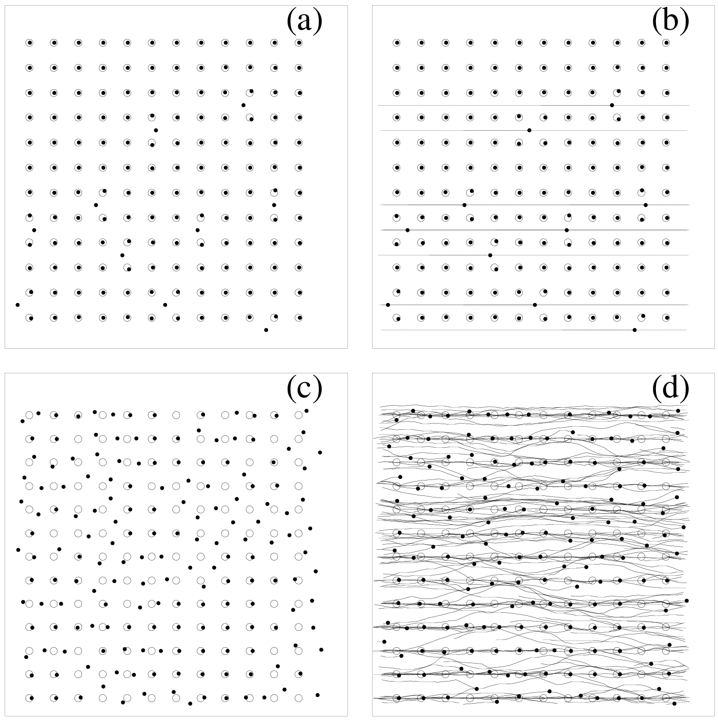
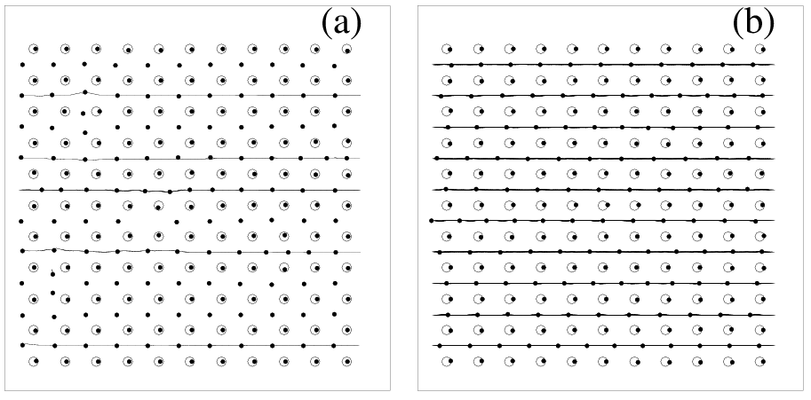
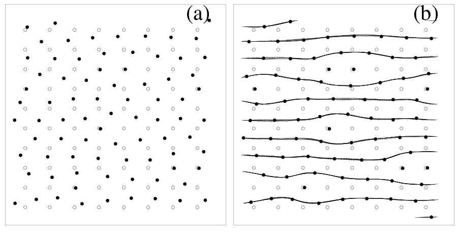
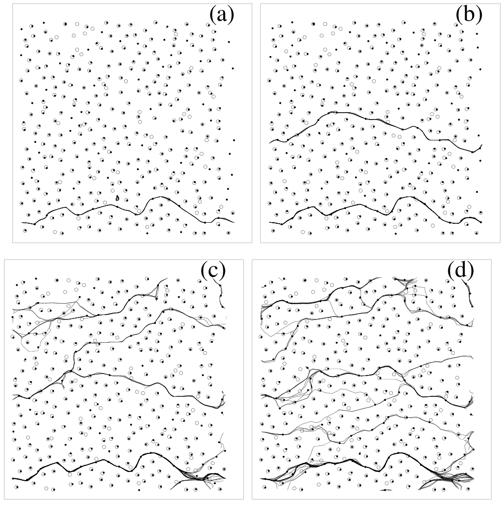
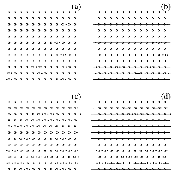
Physical Review B 58, 6534 (1998)

Nonequilibrium Dynamic Phases and Plastic Flow of Driven Vortex Lattices in Superconductors with Periodic Arrays of Pinning Sites

C. Reichhardt, C. J. Olson, and Franco Nori
Department of Physics, The University of Michigan, Ann Arbor, Michigan 48109-1120

(Received 29 December 1997)

We present results from an extensive series of simulations and analytical work on driven vortex lattices interacting with periodic arrays of pinning sites. An extremely rich variety of novel dynamical plastic flow phases, very distinct from those observed in random arrays, are found as a function of an applied driving force. Signatures of the transitions between these different dynamical phases appear as very pronounced jumps and dips in striking voltage-current V(I) curves that exhibit hysteresis, reentrant behavior and negative differential conductivity. By monitoring the moving vortex lattice, we show that these features coincide with pronounced changes in the microscopic structure and transport behavior of the driven lattice. For the case when the number of vortices is greater than the number of pinning sites, the plastic flow regimes include a one-dimensional (1D) interstitial flow of vortices between the rows of pinned vortices, a disordered flow regime where 2D pin-to-pin and winding interstitial motion of vortices occurs, and a 1D incommensurate flow regime where vortex motion is confined along the pinning rows. In the last case, flux-line channels with an incommensurate number of vortices contain mobile flux-discommensurations or "flux solitons", and commensurate channels remain pinned. At high driving forces, the 1D incommensurate paths of moving vortices persist with the entire vortex lattice flowing. In this regime, the incommensurate channels move at a higher velocity than the commensurate ones, causing incommensurate and commensurate rows of moving vortices to slide past one another. Thus there is no recrystallization at large driving forces. Moreover these phases cannot be described by elastic theories. Different system parameters produce other phases, including an ordered channel flow regime, where a small number of vortices are pinned and the rest of the lattice flows through the interstitial regions, and a vacancy flow regime, which occurs when the number of vortices is less than the number of pinning sites. We also find a striking reentrant disordered-motion regime in which the vortex lattice undergoes a series of order-disorder transitions that display unusual hysteresis properties. By varying a wide range of values for the microscopic pinning parameters, including pinning strength, radius, density, and the degree of ordering, as well as varying the commensurability of the vortex lattice with its pinning substrate, we obtain a series of interesting and novel dynamic phase diagrams which outline the onset of the different dynamical phases. We show that many of these phases and the phase-boundaries can be well understood in terms of analytical arguments.
I. INTRODUCTION
A. Lattice driven on a disordered substrate
B. Lattice driven over a periodic substrate
C. Tunable commensurability
D. Nonequilibrium dynamic phase diagram
E. Overview
II. SIMULATION AND PARAMETERS
A. Model
B. Parameters
III. VOLTAGE-CURRENT CHARACTERISTICS AND PLASTIC FLOW REGIMES
A. Interstitial 1D vortex channels
B. Phase boundary I-II
C. Disordered 2D vortex motion
D. Phase boundary II-III: interstitial and disordered flow phases
E. Flux soliton motion in incommensurate 1D vortex channels
F. Phase boundary III-IV
G. Large driving plastic flow phase: IV-V phase boundary
IV. DYNAMIC PHASE DIAGRAM FOR VARYING PINNING FORCE
A. Onset of phase II
B. Onset of phase III
C. Onset of phase IV
V. HYSTERETIC VOLTAGE-CURRENT RESPONSE
VI. EFFECTS OF APPLYING A TRANSVERSE FORCE
VII. DYNAMIC PHASE DIAGRAM AS A FUNCTION OF COMMENSURABILITY
A. Above the first matching field: Bϕ < B < 2Bϕ
B. Second matching field: B = 2Bϕ
C. Above the second matching field: B > 2Bϕ
D. At commensurability: B = Bϕ
E. Below commensurability: B < Bϕ
VIII. DYNAMIC PHASE DIAGRAM AS A FUNCTION OF PINNING RADIUS
A. Dynamic "peak" effect
B. Dynamic "winding interstitial" phase
C. Hysteresis for winding interstitial phase IX
IX. DYNAMIC PHASE DIAGRAM FOR GRADUALLY VARYING THE DEGREE OF DISORDER
A. Formation of vortex channels in samples with a random distribution of pins
B. Vortex "turnstile" motion near 1D flow winding channels
C. Formation of multiple and intermittent channels
X. DYNAMIC PHASE DIAGRAM FOR VARYING DENSITY OF PINNING SITES
XI. VORTEX DYNAMICS ON A TRIANGULAR PINNING ARRAY
XII. SUMMARY
References

I.  INTRODUCTION

A.  Lattice driven on a disordered substrate

Many condensed matter systems can be understood in terms of a periodic elastic lattice driven over a disordered rigid substrate. These systems include flux line lattices in superconductors [1,2,3,4,5,6,7,8,9,10,11,12,13,14,15,16,17,18,19,20,21,22,23,24,25,26], Josephson junctions [36], charge-density-waves [37,38], magnetic bubble arrays [39], Wigner crystals [40], and models of friction [41]. Recently, intense interest has focused on the onset of motion, dynamic phases, and topology of lattices as a driving force is increased. For superconducting systems, experimental work in neutron scattering [17], voltage-current V(I) measurements [18,19,20,21,22,23] and decoration experiments [24,25], as well as theoretical work [5,6,26,27,28,29,30,31,32,37], have suggested that, as an external driving force on the lattice is increased, three distinct dynamical phases appear: a pinned or immobile phase, an amorphous plastic flow phase, and at high drives an ordered uniform flow phase. The plastic flow phase begins at the onset of depinning when portions of the lattice break away and become mobile while other portions remain pinned. The flow-paths at this stage are characterized by winding channels or percolation-like paths [4,6,10,14,33]. Due to the breaking and tearing during this phase, the vortex lattice can become very disordered. As the external driving force is further increased, larger portions of the lattice become mobile until, for high driving, the entire lattice enters a uniform flow stage in which the vortex lattice is much more ordered than in the plastic flow or pinned regimes.
These different flow phases have permitted the construction of a dynamic phase diagram as a function of pinning parameters, temperature, and driving force [6,13,27,31,32]. Similar results have been obtained for charge-density-wave systems [37,38]. It has been suggested that the onset of ordering at the uniform flow phase is sudden and represents a true phase transition to a moving solid or crystal with long-range order [6]. Recently, other studies have suggested that this is not the case and that the driven lattice is instead a highly ordered moving glass [27,28,31,32,37]. Transitions in the dynamical behavior of the vortex flow are believed to be directly related to the peak effect [18,19,20,21,22,23] where a transition to plastic flow is marked by a sudden enhancement of the critical current just below Hc2(T), near the vortex melting point.

B.  Lattice driven over a periodic substrate

Although dynamical transitions have been examined in superconducting systems where the pinning is random, they have not yet been carefully studied in systems with periodic pinning where very different dynamics are expected due to the symmetry of the underlying pinning and the tunability of the disorder. Periodic pinning occurs in numerous superconducting systems such as wire networks [42,43], Josephson junctions [44,45] and layered superconductors [46,47]. High-Tc samples contain other forms of periodic pinning such as that produced by the periodic copper-oxide planes [48].
Recently, increasing attention has focused on samples with lithographically created well-defined periodic pinning structures such as a lattice of microholes [34,49,50,51,52,53,54,55,56] or magnetic dots [57]. In such samples the microscopic parameters of the pinning, such as the size, depth, periodicity, and density, can be carefully controlled. Using Lorentz microscopy techniques [34,56], it has been possible to directly image a vortex lattice interacting with periodic arrays of pinning sites, revealing very interesting commensurability effects in the vortex configurations and dynamics.
Extensive work has been done on the interaction of vortices with a periodic egg-carton potential as in wire networks and Josephson-junction arrays. However, the dynamics of vortices in such systems differs significantly from the case of vortices in periodic pinning arrays we consider in this work. In our system the radius of the pinning sites can be made much smaller than the period of the pinning lattice, permitting interstitial vortices to appear. The distinctive interstitial vortex motion is not found in superconducting wire networks and Josephson-junction arrays. Periodic pinning arrays may also be of technological importance since the arrays can produce higher critical currents than an equal number of randomly placed pins [10,11]. This enhancement of critical currents using periodic arrays has recently been demonstrated for high-Tc systems [55].

C.  Tunable commensurability

A particularly interesting aspect of periodic pinning arrays where the pin radius is small compared to the lattice spacing and where there is only one vortex per pinning site is that disorder can be fine tuned by changing the commensurability. At B/Bϕ = 1, where Bϕ is the field at which the number of vortices equals the number of pinning sites, the vortex lattice is expected to be locked into the periodic pinning array. For B/Bϕ > 1, the vortex lattice can be thought of as containing two species of vortices: the pinned vortices that are commensurate with the array of pins, and the generally more weakly pinned interstitial vortices that are caged by vortices at the pinning sites. The very different dynamical behaviors of these two species has been observed both when the vortices are current-driven [53] and when they are field-gradient-driven [10,11,51,52]. These different dynamics have also been directly observed with Lorentz microscopy techniques [56]. The effect of interstitial vortices at B/Bϕ > 1, as well as the commensurate effects at B/Bϕ = 1, are also of major importance in systems with randomly placed columnar pins, where theoretical [10,58] and experimental [59,60] magnetization studies have shown a substantial drop in the critical current associated with the appearance of interstitial vortices.
It is also possible to have a well defined number of vacancies in the vortex lattice when B/Bϕ < 1. Here, the vortex lattice can be thought of as containing two species of vortices, where the second species, the vacancies, may have different dynamical properties than the first species, the commensurate vortices. This situation and terminology is reminiscent of the case of electrons and "holes" in semiconductors.

D.  Nonequilibrium dynamic phase diagram

In order to observe the dynamics of current-driven lattices near commensurability interacting with a periodic array of pinning sites, we have performed a large number of current-driven molecular dynamics (MD) simulations in which we examine experimentally realizable parameters. Our work is distinct from previous current-driven simulations in that we specifically examine the effects of periodic pinning arrays rather than random arrays. Further, our work covers a much larger range of the microscopic pinning and system parameters than used in previous MD simulations, allowing us to construct a variety of detailed dynamical phase diagrams. A much shorter and less detailed account of some the results presented here can be found in [13].
We find that a vortex lattice driven on a periodic array of pinning sites exhibits far richer and more complex dynamical phase diagrams than the diagrams produced by systems with random pinning arrays. We observe numerous novel plastic flow states and vortex lattice structures distinct from those observed in random pinning arrays. For a certain range of parameters and when the driving force is increased, we find that there is a counter-intuitive drop in the number of mobile vortices as the system undergoes a transition from one plastic flow phase to another. This drop in the number of mobile vortices also implies a negative-differential conductivity, a property that is found in several technologically important semiconductor devices.
We find that the vortex dynamics is highly dependent on the commensurability effects. When B/Bϕ > 1, the interactions between commensurate vortices and interstitial vortices give rise to a number of interesting phases, while when B/Bϕ = 1, a Mott insulator-like phase arises [62]. By systematically disordering the positions of the pinning sites we recover, in the limit of strong disorder, the dynamical phases found in recent theoretical studies of random pinning arrays [4,5,6,10,14,16,26,31,32,33]. For B/Bϕ > 1, and at the onset of depinning in samples with large disorder, we find a distinct "channel phase" where long-lived stable channels, composed predominantly of interstitial vortices, flow around pinned vortices. Such intermittent channel phases where some channels form, freeze and reform have previously been noted in flux-gradient-driven simulations [10,14,33]. A phase with a network of flowing channels is also observed in current-driven samples [5,6,16,26,31,32]. Here, we examine in detail the evolution of the network of vortex channels. In particular, we show that, although some channels are short lived, others are robust under increases of the driving force.

E.  Overview

This work is organized as follows: In section II, we describe the samples used, our numerical algorithm, and the parameters varied. In section III, we show in detail the results for a sample with a square array of pinning sites at a field slightly above commensurability. Current-voltage V(I) curves, individual vortex velocity signals, and images of the vortex motion are presented and correlated with each other, explicitly characterizing the different dynamical phases present.
In section IV we obtain a dynamical phase diagram for the case B > Bϕ and explain many of its features by using force balance arguments which take into account the interactions between interstitial vortices and vortices in the pinning sites.
In section V we show that significant hysteresis is found for certain phases but not for others, and that the hysteresis is not affected by the sample size. Sharp discontinuities in V(I), along with the hysteresis, suggest that some of the dynamical phase transitions are of first order.
In section VI, we demonstrate the existence of a transverse threshold force, as well as the effect of the onset of motion in the transverse direction on the vortex lattice structure. We also show how the transverse force varies with driving force, and discuss the relevance of these results to the recent work by Giamarchi and Le Doussal [28].
In section VII, the V(I) curves and the phase diagram for varying vortex-pin commensurability are presented. We find that the various dynamic phases strongly depend on the commensurability ratio B/Bϕ . For Bϕ < B < 2Bϕ , we observe up to six distinct dynamic phases that arise from the interactions of two species of vortices. For B > 2Bϕ we observe several additional phases. At B/Bϕ = 1 , only two phases are observed, and the critical depinning force reaches its highest level, reminiscent of the so-called "Mott-insulator" phase. For B/Bϕ < 1 , we demonstrate that the initial plastic flow occurs by the motion of vacancies.
In section VIII, we derive the dynamic phase diagram produced when varying the pinning radius. For pins of small radius, we observe a remarkable reentrant disordered dynamic phase. In between these disordered-motion phases there is a channel phase in which the majority of vortices flow in narrow well-defined interstitial channels. This motion is characterized both by a linear Ohmic response in the V(I) curve and by a reduction in voltage fluctuations. We also find that near the boundaries of this channel phase the system exhibits some interesting hysteresis effects. We show the effects of this reentrant behavior on the percentage of 6-fold coordinated vortices in the sample. For certain pinning radii, some transitions among the various plastic flow regimes are marked by a large drop in the number of mobile vortices. We argue that this drop is a force driven dynamical analog of the thermally-driven peak effect observed close to Tc [19,20,21,23].
In section IX, we show the effects on the dynamic phase diagrams of gradually increasing the spatial disorder of the pin array. In the case of large spatial disorder we recover results consistent with studies on totally random pinning arrays. We also present evidence for the existence of distinct regimes of predominantly interstitial channel flow near the initial depinning transition. The characteristics of the channels are also discussed.
In section X we plot the phase diagram for increasing the vortex-vortex interaction strength by means of increasing the vortex density. In section XI we present results for a system with a triangular pinning array. These qualitatively resemble most of the results from the earlier sections, although the flow of vortices in some of the dynamic phases differs from the flow found for the square pinning arrays. In section XII, we summarize our results and discuss their relevance to experimentally realizable systems.

II.  SIMULATION AND PARAMETERS

A.  Model

We model a transverse 2D slice (in the x-y plane) of an infinitely long (in the z direction) parallelepiped with periodic boundary conditions in which stiff vortex lines are parallel to the sample edges (i.e, H = Hz). Inside the sample, the interacting vortices are driven by a Lorentz force over a quenched pinning background. We numerically integrate the overdamped equations of motion:
fi = fivv + fivp + fd = ηvi .
(1)
Here, fi is the total force acting on vortex i , fivv is the force on the ith vortex due to interactions with other vortices, fivp is the vortex-pin interaction force, and fd is the driving force; vi is the net velocity of vortex i and η is the viscosity, which is set equal to unity in this work. The vortex-vortex interaction between two vortices located at ri and rj is correctly modeled by a modified Bessel function. Thus the force acting on a vortex i due to other vortices is
 fivv =   Nv

j=1 
 f0  K1
|rirj|

λ

 
^
r
 

ij 
 .
(2)
Here
f0 = Φ02

2λ3
,
Φ0 = hc/2e is the elementary flux quantum, λ is the penetration depth, Nv is the number of vortices, and rij = (rirj)/|rirj| . The force between two vortices decreases exponentially at distances larger than λ, and we cut off the then negligible force for distances greater than 6λ. We also place a cutoff on the logarithmic divergence of the forces for distances less than 0.1λ. These cutoffs were found to produce negligible effects on the dynamics for the range of parameters investigated. Throughout this work forces are measured in units of f0, lengths in units of λ, and fields in units of Φ02.
The pinning is modeled as Np short-range parabolic wells located at positions r(p)k. The total force on a vortex from other vortices and pinning is
fi
=
  Nv

j=1 
 f0  K1
|rirj|

λ

 
^
r
 

ij 
+
Np

k = 1 
fp

rp
 |rirk(p)|  Θ
rp − | rirk(p) |

λ

 
^
r
 
(p)
ik 
 .
(3)
Here, Θ is the Heaviside step function, rp is the range of the pinning potential, fp is the maximum pinning force of each well, measured in units of f0, and r(p)ik = (rirk(p))/|rirk(p)| . The pinning sites are placed in periodic arrays with a lattice constant a.
The driving force fd is modeled as a constant force which is slowly increased or decreased linearly with time.
In implementing the parallelization of the code we take advantage of the cut-off in the vortex interaction range. Using a one-dimensional domain decomposition, we divide the simulation sample into strips that are multiples of the interaction range in width. Each strip is placed on a separate node, and message-passing techniques [61] are used at the processor boundaries. Since the vortex-vortex interaction has a finite range, any one strip only needs to communicate with its two neighboring strips. Due to periodic boundary conditions the code is run on an even number of nodes. Load balancing is simplified by the repulsive nature of the vortex interaction which tends to spread the vortices evenly among the processors. With flexible domain decomposition the number of processors can be varied without affecting the results. The code is run on a IBM SP parallel computer.

B.  Parameters

We typically increase the driving force by 0.0005f0 every 400 MD-steps for a range of fd ranging from 0 to 0.85f0; using slower rates produces negligible differences. For this work we consider the driving force to be in the x-direction along a symmetry axis of the periodic pinning array. We examine the average of the velocities in the x-direction
Vx = 1

Nv
Nv

i=1 
vi·
^
x
 
(4)
as a function of driving, writing out Vx every 100 to 400 MD steps. This quantity is related to a macroscopic measured voltage-current V(I) curve. Here, Nv is the total number of flux lines in the system.
Since MD simulations are computationally intensive and we wish to vary many parameters in order to investigate several phase diagrams and generate a complete picture of the dynamic phases, considerable effort has been put into optimizing our algorithm. We use a cell-index method as well as force tables for the vortex-vortex and vortex-pin interactions so that excessive function calls are avoided during program execution. More importantly, the simulation also uses a high performance parallel processing technique.
We focus on a system of size 36λ×36λ; however, to study finite size effects, we have also computed several hysteresis runs with system sizes of up to 72λ×72λ. The parameters we vary include the vortex density nv, the pinning site density np, radius rp, strength fp, and spatial distribution. We will consider only the case where the vortex lattice is driven along a symmetry axis of the periodic pinning array. Results for general driving driving angles will be presented elsewhere [15].
We use pinning parameters that are experimentally accessible and are close to those used in recent experiments [51,52]. For the density of pinning sites we have investigated a range from np = 0.1/λ2 to 0.7/λ2, and the corresponding number of pinning sites varies from Np = 130 to Np = 907, respectively. Experiments use samples with a fairly low density of pinning sites, so we focus on a square array with a pinning density of np = 0.25/λ2, as found in the experiments described in [51,52]. We focus on the vortex motion near the first matching field B/Bϕ = 1 , and systematically examine the change in dynamics as B/Bϕ is varied.
In order to separate the different effects that each of the pinning and system parameters (i.e, H, fp, Bϕ) have on the dynamics of the vortices, we fix all the parameters and vary only one in each of the sections of this paper. Moreover, in order to distinguish the effects of disorder caused by the pinning from that caused by thermal effects, we set T = 0. Since we are dealing with square arrays of pinning sites near Bϕ, the ground state vortex configuration is a square lattice commensurate with the pinning sites.
Fig1.png
Figure 1: (a) Vortex and pinning locations for: B/Bϕ = 0.94, fp = 0.625f0, rp = 0.3λ, Bϕ = 0.25 Φ02, and fd = 0. In (b) the same parameters as in (a) are used but now B/Bϕ = 1.06. Vortices are indicated by black dots and pinning sites (which are placed in a square array) are denoted by open circles. In (a) the vortex lattice has three vacancies and no interstitials. In (b) all the pinning sites are occupied and five interstitial vortices can be seen in the areas between the pins.
In Figs. 1(a,b), the positions of the vortices and pinning sites are shown for B/Bϕ < 1, (a), and B/Bϕ > 1, (b). Vacancies appear in Fig. 1(a) and interstitial vortices are present in Fig. 1(b). The initial ground states are obtained in one of two ways. The first is simulated annealing, in which we start from a high-temperature vortex lattice and cool it down. In the second approach, we put down a commensurate vortex configuration and randomly add vortices to the interstitial regions for B/Bϕ > 1 or randomly remove vortices to create vacancies for B/Bϕ < 1. For B near Bϕ, the resulting dynamics are identical using either method.

III.  VOLTAGE-CURRENT CHARACTERISTICS AND PLASTIC FLOW REGIMES

Fig2.png
Figure 2: Average vortex velocity Vx versus driving force fd for B/Bϕ = 1.062, rp = 0.3λ, and Bϕ = 0.25Φ02, with the pinning sites located in a square array and different pinning forces: (a) fp = 0.625f0, (b) fp = 0.37f0, and weak pinning case (c) fp = 0.187f0. The driving force fd is linearly increased slowly from 0 to 0.825f0. In (a) several remarkable jumps in the curve can be clearly seen. These correspond to transitions between different phases in the dynamical behavior of the driven lattice. We have labeled these phases using Roman numerals. In region I the net velocity is 0, corresponding to a pinned phase. In region II, a finite velocity Vx appears and the system exhibits a linear Ohmic behavior. Region III, falling between fd ≈ 0.41f0 and fd ≈ 0.46f0 in (a), has its boundaries marked by sharp jumps in Vx. The fluctuations in the velocities δVx in this phase are much more pronounced than the velocity fluctuations in region II. Phase IV, falling between fd ≈ 0.46f0 and fd ≈ 0.61f0 in (a), corresponds to the 1D incommensurate phase, where both the average velocity Vx and the average velocity fluctuations are smaller than in region III. Phase V corresponds to the phase spanning fd >~0.62f0 in which the entire vortex lattice is moving, but with the commensurate rows moving more slowly than the incommensurate ones. There is no recrystallization at higher driving forces and the vortex motion is always plastic. In (b), for weak pinning the vortex flow goes directly from the pinned phase I to region III, with the interstitial-flow phase II lost. In (c) for even weaker pinning the vortex flow goes directly from region I to region IV, with phases II and III lost.
In Fig. 2 we present a typical series of voltage-current V(I) curves as a driving force fd is slowly increased linearly in time from zero, for samples with B/Bϕ > 1 [illustrated in Fig. 1(b)] and fp = 0.625f0 (a), 0.37f0 (b), and 0.187f0 (c). The strong-pinning V(I) curve in (a) exhibits several remarkable features which can be clearly seen as discontinuous jumps in the net vortex velocity in the x-direction, Vx. In the first part of the curve, as the driving force is increased, the velocity signal is zero, indicating that the vortex lattice is pinned. At approximately fd = 0.146f0, a finite velocity appears due to the depinning of the weakly pinned interstitial vortices, and the V(I) curve becomes linear. At fd ≈ 0.406f0, there is a very sharp jump up in Vx, indicating a sudden increase in the number of mobile vortices. It can be clearly seen that the voltage fluctuations become much larger after this jump. At fd ≈ 0.462f0, we see a sudden drop in Vx and a suppression of the fluctuations in Vx, indicating that the number of mobile flux lines has dropped and is remaining constant in number. Finally, between fd ≈ 0.595f0 and fd ≈ 0.6125f0, which is slightly smaller than the pinning force of each pinning site, fp = 0.625f0, we see another large increase in Vx that continues until the entire lattice becomes mobile. At this point, for fd >~0.625f0, the V(I) signature is linear. Each of these features in the V(I) curve correspond to different vortex flow regimes which we label I through V. Region I is the pinned phase, and phases II through IV are plastic flow phases in which portions of the vortex lattice move while other portions remain pinned. Phase II appears only when fp > 0.37f0, and the range of driving forces over which IV appears increases with increasing pinning strength.
In Fig. 2(b) for a sample with weaker pinning (fp = 0.37f0) phase II is lost and the vortex flow jumps directly to phase III. There is also no sharp discontinuity in the transition from phase II to phase III; however, the transition from region III to region IV still shows a discontinuity. The onset of phase V now occurs at fd = 0.37f0 = fp. In Fig. 2(c) for a sample with even weaker pinning, (fp = 0.187f0), both region II and region III are lost. The vortex flow goes directly from phase I to IV and jumps to phase V at fd = 0.187f0. Region V is the homogeneous flow phase where the entire vortex lattice is flowing but doing so plastically.
Fig3.png
Figure 3: Snapshots (left panels) and trajectories (right panels) of the vortex lattice for phases II (1D interstitial channels) and III (disordered flow) of Fig. 2(a). The vortices are represented by black dots and pinning sites by open circles. The trails, where the vortices have been moving eastbound along the x-direction, are indicated by the trajectory lines on the right panels. (a) A snapshot of the vortex lattice in phase II with 10 interstitial vortices; note the similarity with the lattice structure in the pinned region I, shown in Fig. 1(b). (b) Region II corresponds to the 1D motion of interstitial vortices between the pinning rows. In (c-d) the strikingly different vortex structures and flow paths of region III can be seen. Here the vortex lattice is no longer square but is disordered, with vortices moving in and out of the pinning sites. The flow paths in (d) now wind in a disordered manner in both the x and y directions. Further, it can be seen from the trails that vortices are now jumping in and out of the pinning sites.
Fig4.png
Figure 4: 
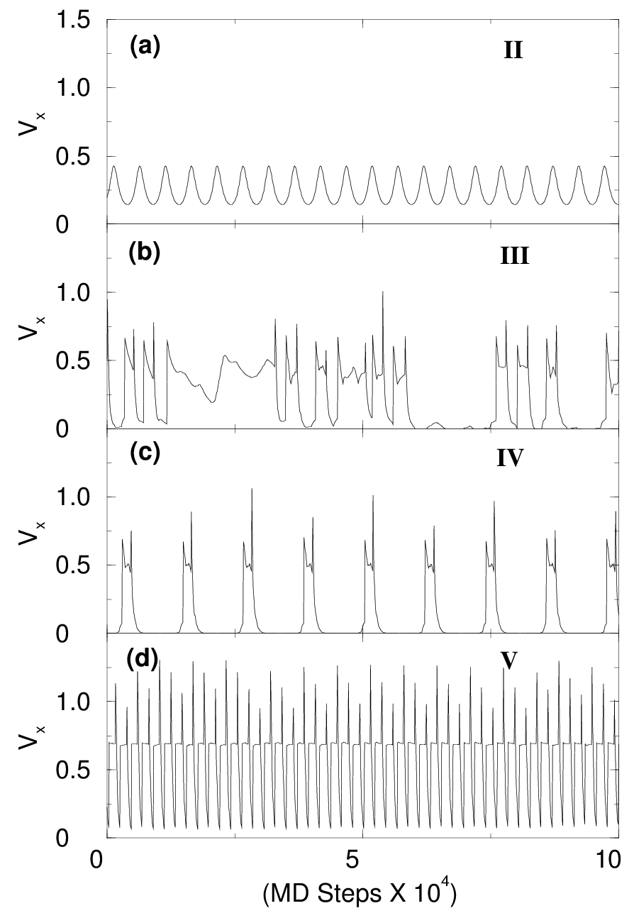
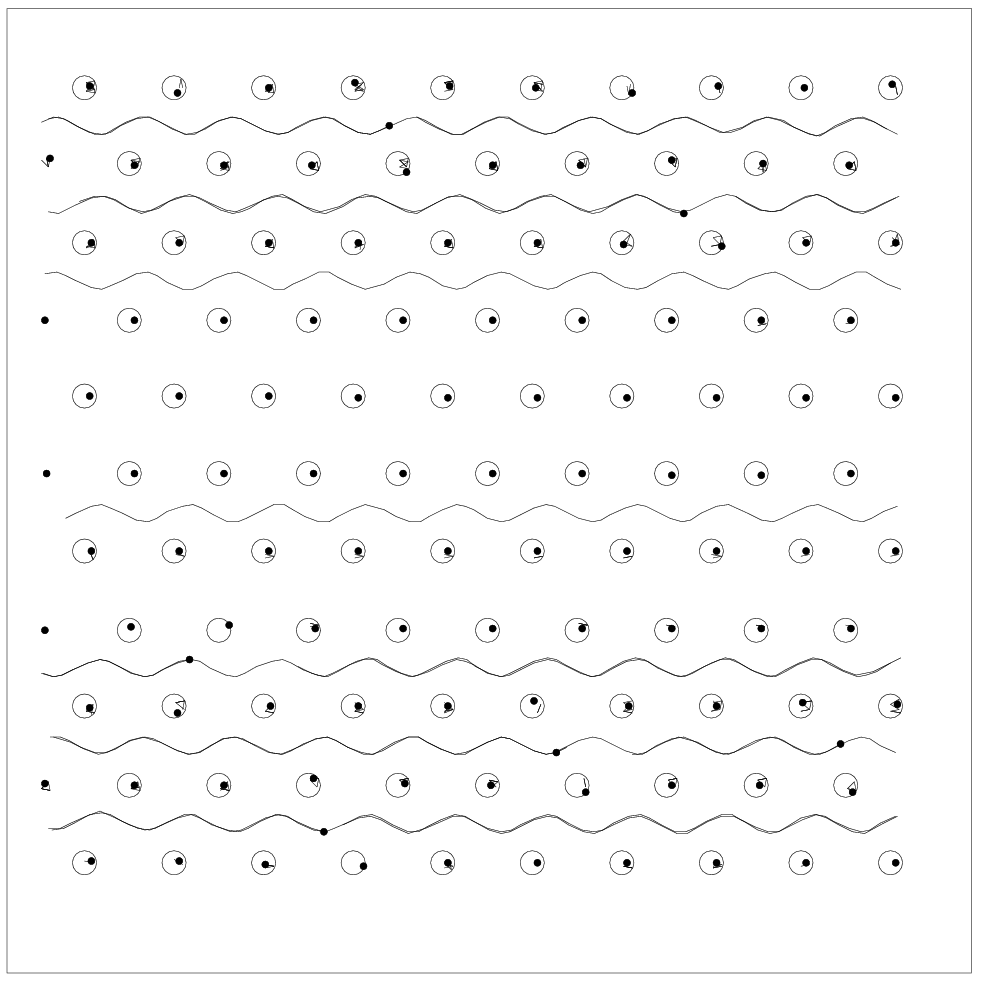
Snapshots (left panels) and trajectories (right panels) of vortices for regions IV (1D incommensurate flow) and V (incomm. and commensurate plastic flow) of Fig. 2(a). In (a,b) we can see that the vortex lattice structure and flow patterns are quite different from those shown in Fig. 3. 
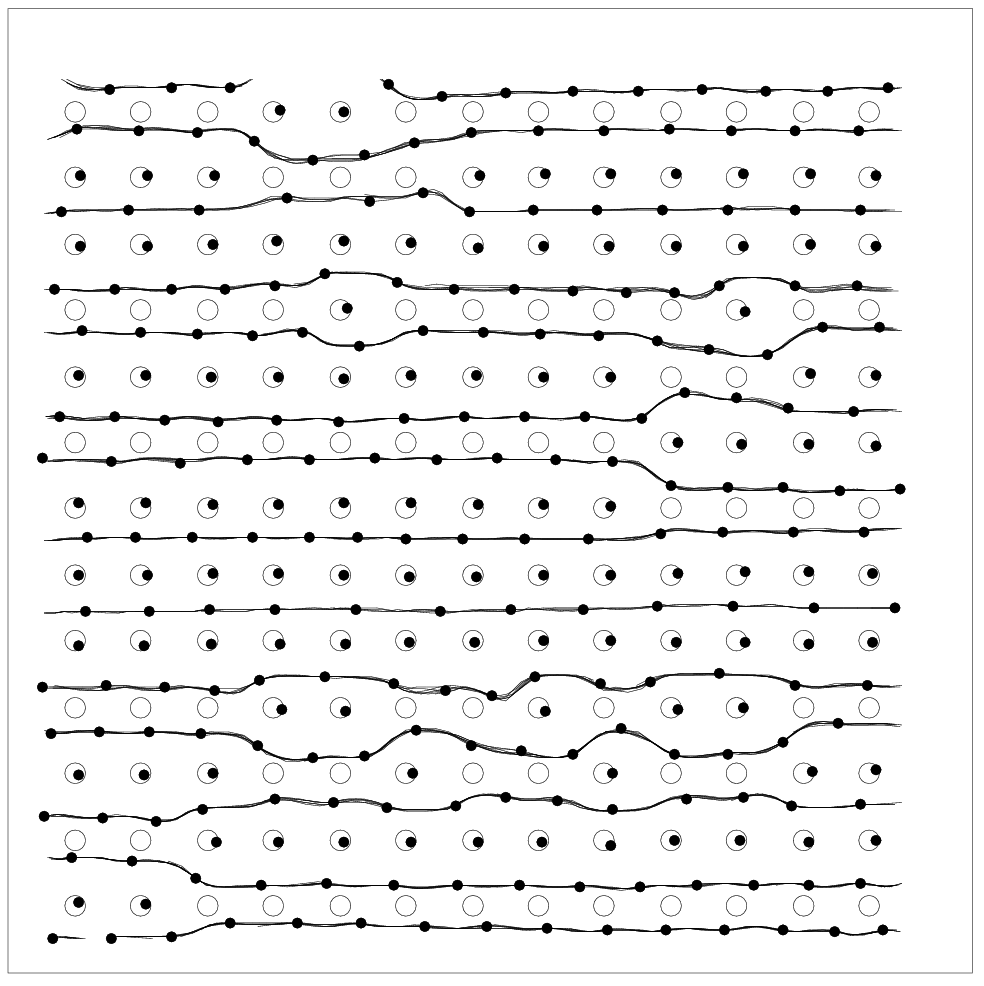
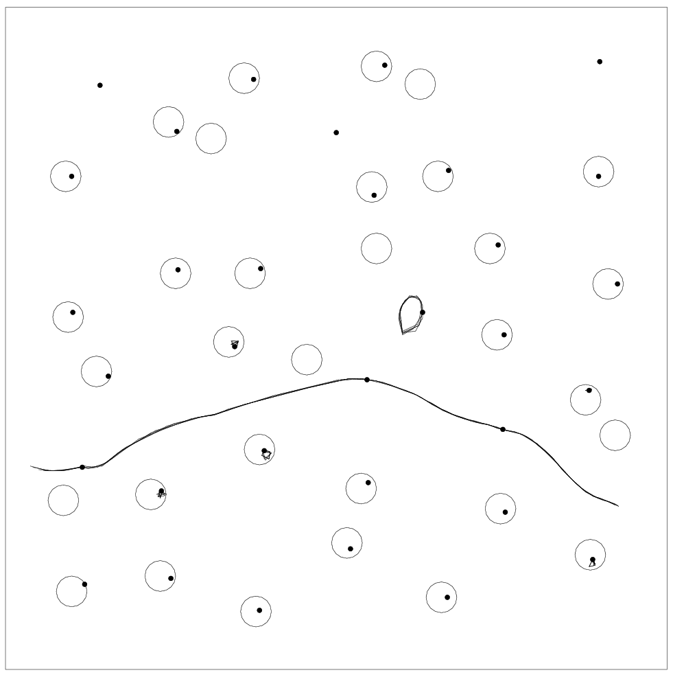
In (a) vortices are now aligned with the pinning rows, with certain rows forming 1D incommensurate structures. In (b) it can be seen that the motion in region IV is 1D, but unlike the interstitial flow in phase II, where the vortices flowed between the pinning rows, the vortices now flow along the pinning rows. 
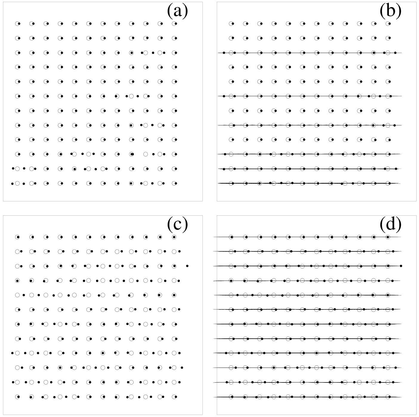
Rows containing an incommensurate number of vortices (i.e., where there are more vortices than pinning sites) are the only places where motion is occurring, while rows with a commensurate number of vortices remain pinned. In particular, note that the first, second, fourth, seventh, and ninth (commensurate) rows from the top edge remain pinned while the remaining incommensurate rows slide past the commensurate ones. Flux motion in phase IV, shown in (b), occurs through mobile vortex discommensurations. These "flux-solitons" propagate at a faster speed than the actual vortices.
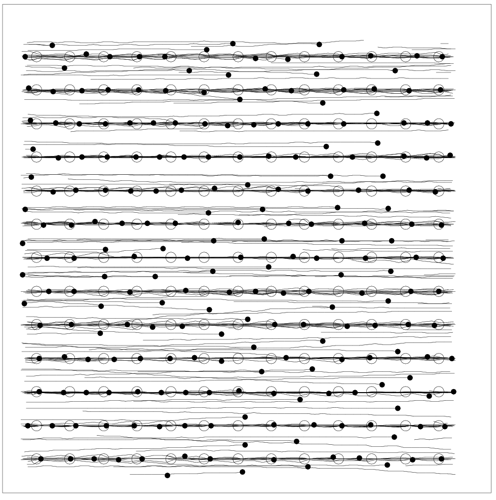
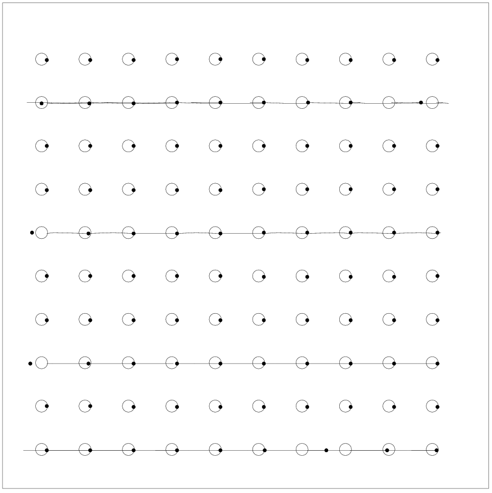
 In (c,d) the entire vortex lattice is moving in 1D paths along the pinning rows, corresponding to phase V. The vortex lattice in (c) is not triangular, but is similar to that seen in phase IV. The defects caused by the incommensurate vortices (discommensurations or flux solitons) do not heal out since vortex motion in the transverse direction does not occur in regions IV and V. The incommensurate rows are more mobile than the commensurate rows so they slip past the commensurate rows; thus the vortex motion is always plastic.
Fig5.png
Figure 5: The velocity of an individual typical vortex in a system with the same parameters as in Fig. 2(a). In (a) an interstitial vortex in phase II moves with a velocity periodic in time caused by its interactions with pinned vortices that form a periodic barrier to motion. The velocity of the interstitial vortex is never zero. In (b) a typical vortex in phase III has a disordered motion, with intervals of time where the velocity is zero (when the vortex is pinned) interrupted with times when the vortex is moving. In (c) a vortex in a row with an incommensurate number of vortices moves in short periodic pulses. During each pulse or soliton the vortex moves only one pinning site, and it is pinned between pulses. The period of the vortex soliton pulses are much longer than the period observed in the motion of phase II [shown in (a)] since in (c) the periodicity arises from a pulse traversing the entire sample, rather than from a vortex moving between two pinning sites. In (d) a vortex in a row with an incommensurate number of vortices again moves periodically along the pinning row, but the velocity never drops to zero since the vortex is never totally pinned.
To show explicitly that the features in the V(I) curves correspond to different nonequilibrium dynamical flow phases, in Figs. 3 and 4 we show a series of snapshots of the vortex positions (left panels) as well as trajectory lines (right panels) indicating where the vortices have flowed during a short period of time for regions II through V of the voltage-current curve in Fig. 2(a). The vortex lattice structure for region I, where the applied driving force is too weak to depin any vortices, is shown in Fig. 1(b). In Fig. 5(a-d) plots of the velocity of an individual vortex versus time for regions II-IV also show the very different types of vortex dynamics present in each phase. It is important to point out that the vortices in interstitial locations are pinned by the magnetic-repulsion caging effect of the vortices trapped at pinning sites.

A.  Interstitial 1D vortex channels

Figure 3(a) presents a "snapshot" of the vortex locations at a single instant in region II of the voltage-current curve. This figure shows that the mobile interstitial vortices are located between the rows of pins. The vortex lattice structure is essentially the same for regions I and II. To approximate the percentage of flux lines which are mobile at a specific driving force, we define the following measure based on the net velocity in the x-direction,
σ = Vx

|fd|
 ,
(5)
For region I, σ has a value of σ = 0.06, indicating that only the interstitial vortices are mobile since the percentage of vortices above Bϕ is also (BBϕ)/Bϕ = 0.06. Figure 3(b) shows the flow in region II of the V(I) curve with outlines of the paths the vortices have followed. This confirms that only the interstitial vortices flow in region II and that the motion is constrained to move in 1D channels between the rows of pinning sites due to the square symmetry imposed by the pinned vortices. Figure 5(a) shows that the velocity of the mobile vortices is never zero and that it has an oscillatory component [65] since the energy landscape imposed by the vortices pinned at the pinning sites has the same square periodicity as the pinning array.

B.  Phase boundary I-II

For the case of strong pinning when region II exists, as in Fig. 2(a), we can make a simple estimate of the threshold driving force needed to depin an interstitial vortex by considering the balance of forces when there are two species of vortices, interstitial and pinned. An interstitial or incommensurate vortex will feel a force from commensurate pinned vortices fincc = fincommcomm, forces from other interstitial vortices fincinc, and the driving force fd. An interstitial vortex will thus remain immobile as long as
fincc + fincinc + fd = 0.
For the case when there are few interstitial vortices, as in Fig. 2(a), we consider only the interactions with the commensurate pinned vortices and the driving force and neglect the interactions between pairs of incommensurate vortices. When there is no driving force the interstitial vortices sit in the center of the interstitial locations, and each has four nearest neighbor commensurate pinned vortices. As the driving force is increased the interstitial vortex will start to shift in the interstitial location and experience a restoring force from the commensurate pinned vortices. Since the vortex interactions decay exponentially with distance, the dominant restoring force on an interstitial vortex comes from the four nearest commensurate pinned neighbors. The maximum restoring force occurs when the interstitial vortex has shifted halfway between its zero driving position and the pinning site. An estimate for the threshold force is

fd
=
2f0 K1 
√5a


 cos(arctan(2))
2f0 K1 


13
 
a


cos(arctan(2/3)).
(6)
Using this equation with the parameters from Fig. 2(a) we find that onset of region II should occur at a driving force of fd = 0.14f0, which is in very good agreement with the value of fd = 0.146f0 obtained from the simulations.

C.  Disordered 2D vortex motion

In Fig. 2(a), at the onset of region III we find a significant jump in Vx indicating a sudden increase in the number of mobile flux lines. The approximate percent of mobile vortices is now σ = 0.44, which indicates that vortices are now being depinned from the pinning sites since the percentage of vortices above Bϕ remains σ = 0.06. Significant fluctuations for phase III in the V(I) curves can be seen, indicating that the number of mobile flux lines is rapidly fluctuating. Figure 3 presents the vortex positions (c) and trajectories (d) for region III of Fig. 2(a). We see that the vortex lattice structure and flow pattern is of a remarkably different nature than that observed in the interstitial flow phase II. The vortex lattice has now become disordered, and the vortex trajectories are no longer 1D but move in both the x and y directions. It can be seen that some pin-to-pin vortex motion now occurs. Unlike the motion in phase II, where only the interstitial vortices move and vortices at the pinning sites remain pinned, all the vortices in region III take part in the motion with any one vortex moving for a time and then being temporarily trapped. Figure 5(b) shows the velocity of a single vortex in region III. The velocity is not periodic as in phase II, Fig. 5(a), but shows irregularities, including sharp bursts followed by periods of no motion.

D.  Phase boundary II-III: interstitial and disordered flow phases

To understand the crossover from the 1D interstitial flow phase II to the disordered 2D flow region III, we consider the balance of forces in a sample with two kinds of vortices, interstitial and pinned, just as in the crossover from region I to region II. Interstitial vortices exert a force fincc = fincommcomm on a commensurate vortex (denoted by the sub-index c) while commensurate vortices exert a force fcc on this vortex. In the simple case when there are no interstitial vortices, commensurate vortices stay pinned as long as fd < fp. When interstitial vortices are present, they move between the rows of the lattice of pins and exert an additional force on the pinned vortices, resulting in an earlier depinning transition. A commensurate vortex at a pinning site remains pinned by the force from the pinning site as long as the following force balance inequality holds:
|fp| > |fd + f incc + fcc| .
(7)
Due to the symmetry of the underlying pinning lattice, it is clear that the net force from the other commensurate vortices will be fcc = 0 when every pin is occupied by a vortex (or for other symmetrical configurations). Since fincc is the sum of all the interactions from mobile interstitial vortices, fincc is time-dependent and has a complicated form.
Fig6.png
Figure 6: Schematic diagram showing how the interstitial vortices depin the commensurate vortices. The interstitial vortex i is at its closest distance, approximately a/2 + rp/2, to the pinned vortex j. Notice that vortex j moves an additional distance, which we approximate as rp/2, from the center of the parabolic pinning well due to the force from vortex i. When fd is large enough, vortex i will be able to depin vortex j, producing a transition from one type of plastic-flow (type II or interstitial 1D flow) to another (type III or disordered 2D flow).
To estimate fincc, we consider the case where B is only slightly higher than Bϕ. Here, the interstitial vortices are on average sufficiently far apart that we can estimate fincc from a single interstitial vortex interacting with commensurate vortices as it moves between the pinning rows. The force exerted by this interstitial vortex i on a commensurate vortex j has a maximum value when the interstitial vortex reaches the point of its closest approach to the pinned vortex, which for a square lattice occurs when the interstitial vortex is aligned with a column of pinning sites (see Fig. 6). The distance between vortices i and j at closest approach is rij = a/2, or half the pinning lattice spacing a. We also take into account the fact that the pinned vortex will be shifted slightly from the center of the well both because of the applied driving force and because of the repulsion from the interstitial vortex. This adds a small distance, which we approximate as rp/2, to the distance between the interstitial vortex and the pinned vortex, giving a total "distance of closest approach" of approximately rija/2 + rp/2. In Fig. 6 a schematic diagram of this is presented. In terms of magnitudes, a commensurate vortex remains pinned as long as the following inequality holds:
fp >   ⎛


fd2 + fij2
a + rp

2

 
(8)

fp >
fd2 + f02 K12
a + rp


1/2

 
 ,
(9)
where fij = f0K1(rij/λ) is the force between the interstitial vortex i and the commensurate vortex j. Driving forces which satisfy this inequality result in phase-II-type interstitial flow. As the driving force fd is increased, the inequality eventually ceases to hold, and an interstitially moving vortex can cause vortices in the pinning sites to depin. These depinned vortices move away with some component of their velocity in the transverse y direction. As these vortices move, they depin additional vortices in an irregular fashion, thus producing the transition to the disordered 2D-flow phase III. As long as fp < fd, the vortices in the sample can be temporarily trapped; therefore, not all of the vortices move simultaneously.
We predict that the transition from 1D interstitial to disordered 2D flow (i.e., from phase II to phase III in Fig. 2(a)) should occur when the inequality in (9) no longer holds. To verify this prediction we consider a sample with parameters equal to the ones presented in Fig. 2(a); namely: a = 2.0λ, rp = 0.3λ, and fincc = f0 K1(1.15) = 0.4695f0 . The upward jump in Vx, signaling the transition between phases II and III, occurs at fd = 0.406f0. Using inequality (9), we find that the jump will occur at this value of fd if fp = 0.621f0. This is in very good agreement with the input value of fp = 0.625f0 used for the simulations shown in Fig. 2(a). The fact that the calculated value is somewhat less than the actual value is probably due to the interactions of other interstitial vortices which were not taken into account in inequality (9).

E.  Flux soliton motion in incommensurate 1D vortex channels

Upon further increasing the driving force fd in Fig. 2(a), we observe a new nonequilibrium dynamic phase, which we label region IV. At the onset of this phase, a surprising sharp drop in Vx occurs, indicating a decrease in the number of mobile vortices. In particular, we find that a fraction σ ≅ 0.24 of the vortices are mobile, significantly lower than the fraction, σ ≅ 0.44, that were mobile in phase III.
In Fig. 4(a,b), we see that the vortex motion possesses a very different structure and flow pattern from that of the 1D interstitial flow of phase II and the random flow of region III. The flow in phase IV is entirely 1D with the mobile vortices flowing along the pinning rows, which is distinct from the 1D interstitial flow in phase II where mobile vortices flowed between the rows. We observe that the presence of additional vortices in certain rows creates incommensurate 1D structures in the form of discommensurations or flux solitons along the pinning row, and that it is in these rows where motion occurs [65] in the direction of the driving force fd. Rows that are commensurate are immobile. Due to the 1D nature of the incommensurate flow in phase IV, the voltage fluctuations δVx for phase IV are considerably smaller than the δVx's found during the random flow of phase III.
It is interesting to point out that the drop in the fraction of moving vortices at the III-IV transition implies a negative differential conductivity
dV/dI < 0.
This behavior is often observed in semiconductors, and can be useful for certain devices [63].
The appearance of 1D motion exactly along the rows of pins might seem counterintuitive. This is so because for B/Bϕ > 1 and fd = 0, when the vortices are not moving, the only positions for extra vortices that are stable against perturbations in the transverse y-direction caused by other interstitial vortices are the interstitial positions between the rows of pinning, as in Fig. 1(b). For moving vortices, the situation is quite different because the extra vortices in incommensurate rows spend part of their time in the pinning sites. The pinning sites create a stabilizing force against perturbations in the transverse y-direction, so that motion becomes confined to the pinning rows along the longitudinal direction. The vortex motion occurs only where one or more incommensurate vortices are located along the row. As the disturbance or flux soliton moves, it causes the vortex in front of it to depin and then this one moves to a point where it will depin the next vortex. From direct observations of the flux motion, as in Fig. 4(b), we find that every discommensuration is composed of four mobile vortices. The periodic-pulse nature of the discommensuration flow is clearly seen in Fig. 5(c) where the individual velocity of a single vortex in region IV from Fig. 2(a) is plotted. An individual vortex moves only for a short time as the discommensuration moves through and then is pinned again. Using the parameters presented in Fig. 2(a), where a fraction (BBϕ)/Bϕ = 0.06 of the vortices are incommensurate, we find that the total fraction of mobile vortices is about four times higher, or σ = 0.24.

F.  Phase boundary III-IV

In order to understand when incommensurate vortex motion along the pinning rows, as seen in phases IV and V, is stable, we construct a simple force-balance argument. We consider a force fy in the transverse y-direction that deflects a vortex away from its longitudinal motion along the pinning row in the x-direction. Suppose that under the influence of this force fy, the vortex moves a distance dy in the transverse y-direction equal to rp , the pinning radius, in time t. Thus,
dy = fy t = rp   .
(10)
For a particular driving force fd in the longitudinal x-direction, if a vortex can move a distance dx in the x-direction equal to the pinning lattice constant, a, within the same time t = dy/fy, the vortex will feel a pinning force in a direction opposite to fy that pulls the vortex back into the row a distance:
dx = fd t = a.
(11)
We note that in actuality the vortex only spends a finite amount of time in the pinning site so it is not pulled all the way to the center of the pinning site; however, for convenience we assume here that the vortex is pulled all the way to the center. From Eqs. (10) and (11) it can be seen that motion along the row is stable if
fy < fd rp

a
 .
(12)
For example, for the parameters in Fig. 2(a), with rp = 0.3λ and a = 2.0λ, if the vortex lattice is being driven with a force of fd = 0.5f0 in phase IV with incommensurate 1D channels on pin rows, the 1D motion is stable against perturbations of size fy < 0.075f0. Note that inequality (12) indicates that as the size of the pinning sites is increased (i.e., increasing rp) or the pinning density is increased (i.e., decreasing a) motion along the rows will be more stable. Inequality (12) also erroneously predicts that fy increases linearly with fd; however, the maximum possible value for fy for stable vortex motion is fp.
Fig7.png
Figure 7: Schematic diagram showing how interstitial vortices depin commensurate vortices at pinning sites at the onset of the dynamic phase IV (incommensurate 1D flow). The interstitial vortex i at the center of an interstitial site depins vortex j at a distance 2−1/2a + rp.
To derive an expression for the increasing driving force at which region IV appears, we take into account the fact that there is an average energy barrier for interstitial vortices to enter the pinning rows since vortices at pinning sites tend to keep interstitial vortices in between the rows. Once the vortices are in the random-flow phase III, many of the vortices are moving in interstitial regions and (see Section III) these vortices depin vortices at nearby pinning sites. As fd increases, pinned vortices become easier to depin and there is an increase in the distance rmin from which an interstitial vortex can depin a pinned vortex, so that rmin > a/2 + rp/2. When fd is large enough, rmin reaches a limiting value such that a vortex located approximately halfway between two columns of pinning sites can depin one of the vortices in the row ahead of it. A schematic diagram of this situation is presented in Fig. 7. To verify this, we note that a vortex placed at the center of an interstitial site exerts a force approximately equal to fij(a/√2 + rp)cos(45°) in the x-direction on a vortex in a pinning site. As a function of the driving force fd, the pinning force fp needed to keep a vortex pinned at a pinning site when an interstitial vortex is located at the center of an interstitial site is
fp >

fd + fij
a

√2
+ rp
/√2
2

 
+ fij2

2

a

√2
+ rp

1/2

 
(13)

fp
>
 

fd + f0

√2
K1
a

√2λ
+ rp

λ


2

 
+
f02

2
K12
a

√2λ
+ rp

λ


1/2

 
(14)
After an interstitial vortex depins a commensurate vortex, it experiences a net force toward the vacated pinning site from the other pinned commensurate vortices. It must travel an approximate distance a/2 in the x-direction before it is adjacent to the just vacated pinning site. During this time, however, the depinned vortex also moves a distance a/2 in the x-direction as well as a/2 in the y-direction and in principle should itself be able to depin another commensurate pinned vortex. The original interstitial vortex is just far enough from the first depinned vortex that it is able to be trapped by the vacant pinning site.
Thus, when fd is large enough, vortices moving in the random 2D flow regime (phase III) will start to become confined along the horizontal pinning rows and, provided that inequality (12) is met, this motion along the pinning rows should be stable. Substituting in inequality (14) the parameters used in Fig. 2(a) and the value of fd = 0.406f0 observed at the onset of the 1D incommensurate motion, we find a calculated value of fp = 0.624f0, which is in very good agreement with the actual value fp = 0.625f0 used in the simulations.

G.  Large driving plastic flow phase: IV-V phase boundary

As fd is increased to almost fp, the entire vortex lattice starts to flow in a phase which we label region V. The vortex flow pattern for phase V for the system in Fig. 2(a) is presented in Fig. 4(c,d). The type of motion and vortex lattice structure in region V resembles that of phase IV with vortices moving in 1D channels along the pinning rows; however, in region V all the vortices are mobile. The velocity of an individual vortex is periodic (as shown in Fig. 5(d)) due to the underlying periodic pinning lattice. Individual vortices can slow down considerably but are never completely repinned, as indicated in Fig. 5(d) by the fact the the velocity is always greater than zero.
The transition from region IV-V in Fig. 2(a) is not as sharp as that of II-III and III-IV but instead occurs over the range of 0.595f0 <~fd <~0.613f0. This can be understood by considering that in region IV certain rows contain incommensurate mobile vortices. As these vortices move past pinned vortices in adjacent commensurate rows they will exert a small force in addition to the driving force that causes the adjacent commensurate rows to depin at a driving force lower than fd = 0.625f0.
We also observe that in region V rows with incommensurate numbers of vortices move faster than commensurate rows so that rows with different numbers of vortices slide past one another. Some portions of the vortex lattice can be seen to have triangular order; however, there are portions where this does not hold. A Voronoi analysis gives a probability of 6-fold coordinated vortices of P6 = 0.83. This is less than P6 = 1 because of the presence of the incommensurate rows. As fd is increased further, the density of defects and structure of the vortex lattice do not change. This result is different from simulations [5,6] with random pinning arrays which show that for sufficiently high driving rates, the defects in the vortex lattice heal out and P6 = 0.95.

IV.  DYNAMIC PHASE DIAGRAM FOR VARYING PINNING FORCE

Fig8.png
Figure 8: The dynamic phase diagram for the pinning force fp versus driving force fd with B/Bϕ = 1.062, rp = 0.3λ, and Bϕ = 0.25 Φ02, with a square pinning lattice. Regions I through V correspond to the same dynamical phases shown in Figs. 2(a), 3, and 4. For very weak pinning, fp < 0.1f0, regions II-IV are lost and the vortex lattice flows elastically both along the pinning sites and also in the channels in what we label phase Velastic. The disordered 2D flow phase III first appears at fp ≈ 0.25f0 and phase II at fp ≈ 0.37f0 . The driving force at which a transition from phase I to II occurs saturates at a value of fd ≈ 0.146f0, which corresponds to the force needed to depin an interstitial vortex. As fd is increased, the phase boundaries II-III, III-IV, and IV-V become linear. When the depinning scenario presented in Fig. 7 can take place, the interstitial vortex can occupy the just vacated pin site. This gives rise to the incommensurate 1D flow of phase IV. If fp is strong enough, the interstitial vortex of region II will have to reach maximum proximity to the pinned vortex in order to dislodge it (as shown in Fig. 6). In this case the interstitial vortex cannot occupy the pin site just vacated. Thus its deflection along the transverse direction triggers the type of motion in phase III. For large pinning force fp and medium driving fd, phase II dominates the phase diagram.
In order to better characterize the nonequilibrium dynamic phases, we have performed a series of simulations in which fp is systematically varied, while the rest of the parameters are fixed at the same values used in Fig. 2(a). In Fig. 8 we present the resulting phase diagram where the onsets of different flow behavior can be observed. For very weak pinning, fp < 0.1f0, the features in the flow phases and V(I) curve are lost and the vortex lattice moves elastically. The driving force at which the phase boundary I-II occurs increases with increasing pinning force until the pinning force reaches a value of fp close to the interstitial pinning force, fpinterstitial ≈ 0.146f0. At this point, the value of the driving force at the transition saturates because, although the pinning force fp of the pinning sites is being increased, the vortex-vortex interaction which determines the interstitial pinning force is not changed.

A.  Onset of phase II

Figure 8 shows that the interstitial motion of phase II occurs only when fp >~0.37f0. This can be understood by considering that when fp <~0.37f0, inequality (9) cannot be satisfied for any driving force, so that phase II cannot occur, and thus the boundary between phases I and II stops.
For a pinning force of fp = 0.35f0, an interstitial vortex at closest approach exerts a force f0K1(1.3) = 0.3725f0 on a vortex at a pinning site. This is greater than the pinning force, so as soon as the interstitial vortices move, they cause vortices at the pinning sites to depin, producing phase III motion. In this case, it is not possible for interstitial vortices to move between the pinning rows without depinning vortices trapped at the pinning sites, so the interstitial 1D motion of region II does not occur for these weak pins. Region II occurs in the phase diagram only for values of fp and fd that satisfy both inequality (9) and inequality (14).

B.  Onset of phase III

As fp is increased further, a stronger driving force is required for the interstitial vortices moving in phase II to depin commensurate vortices so that a transition to region III can occur. The phase boundary line separating phases II and III is expected to follow the equation
fp =
fd2 + fij2
a + rp

2


1/2

 
,
(15)
which for large drives fd >> fij(a/2 + rp/2) (15) reduces to the linear relation
fpfd
(16)
in good agreement with the phase diagram in Fig. 8. Phase III occurs for fp and fd values that satisfy inequality (14) but violate inequality (9). Under these conditions, commensurate vortices can be depinned, but phase IV motion is not yet possible.

C.  Onset of phase IV

It is clear from the dynamic phase diagram in Fig. 8 that when fp < 0.25f0, motion begins immediately in phase IV, without passing through phases II and III. For values of fp less than fp = 0.25f0, inequality (14) remains invalid for all driving forces so that the initial motion appears as region IV. For example, for fp = 0.25f0, motion starts at fd = 0.09f0, the right side of inequality (14) is 0.277f0, and the inequality is invalid.
The boundary between phases III and IV satisfies the relation (14). At high drives, inequality (14) behaves as fpfd , in in good agreement with the III-IV boundary in the phase diagram in Fig. 8. Region IV flow occurs in the portion of the phase diagram where both inequalities (9) and (14) no longer hold but fd < fp.
Finally, the phase boundary between regions IV and V follows the linear relation of fpfd. When fd > fp, the flow is 2D and not uniform because rows slide past each other.
We point out that in Eq. (1) we have assumed fd to be uniform on all the vortices, which is the case for thin-film superconductors where λ can be comparable or larger than the system size. Vortices in thin film superconductors will interact via a Pearl-potential fvv  ∼ 1/r rather than the modified Bessel function which we use. The modified Bessel function is appropriate for bulk superconductors. By using these different vortex interactions, the phase boundaries we observe may be shifted slightly but the qualitative features should be the same. For bulk superconductors an applied current will form a gradient in the vortex density. If the pinning is weak, the gradient should be small and the dynamic phases should be the same throughout the sample. For very large flux-gradients different dynamic phases may occur in different regions of the sample. In section VII we show how the dynamic phases are modified when considering samples with different vortex densities.

V.  HYSTERETIC VOLTAGE-CURRENT RESPONSE

Fig9.png
Figure 9: The hysteresis curve for the system presented in Fig. 2(a) as the driving force is brought up to fd = 0.7f0 and then brought back down to fd = 0. Some phase boundaries (IV-III) and (III-II) show hysteresis, while others (V-IV) and (II-I) do not. Boldface Roman numerals refer to phases which appear when ramping up, while unbold refer to the ramp-down process.
To further characterize the driven vortex flow in the presence of periodic pinning sites, we examine hysteresis effects with simulations in which the applied driving force fd is ramped up and then ramped down. Figure 9 shows the hysteresis in the V(I) curve for the sample used in Fig. 2(a). The region labels in Fig. 9 are in boldface for the ramp up and in non-boldface for the ramp down stage. Little hysteresis occurs as the system goes back through phases V and IV except for a small loop in region IV. Region III does not appear on the reverse path at the same value of the driving force at which it appeared when increasing the driving force. Instead, phase IV on the reverse path extends into what is phase II on the forward path, and the vortex lattice only enters region III at fd = 0.34f0, which is below the value fd = 0.41f0 at which region III appears for the forward path.
The fact that phase III appears at all for such a low value of fd may appear to contradict the predictions of inequality (9), which indicates that for fp = 0.625f0, region III can only arise when fd > 0.41f0. Inequality (9) is, however, only valid when there are interstitial vortices moving between the rows of pinning. This occurs for the ramp-up part of the hysteresis curve, when there is a transition from phase II to III. In contrast, when a transition from phase IV to III occurs, the vortices are moving along the pinning rows, so there are no interstitial vortices between the rows, and thus inequality (9) does not apply. It is possible for phase III to appear on the reverse path because the extra incommensurate vortices approach pinned vortices closely since they are moving along the pinning rows rather than between the rows.
Region IV persists for so long on the reverse leg because once the 1D incommensurate channels are formed, there is a barrier to perturbations in the transverse-direction, as noted in section III and by inequality (12). This barrier is examined further in the next section. After region III appears on the reverse path, the vortex motion returns to the interstitial flow type seen in phase II.
The hysteresis and the sharp discontinuities in Vx suggest that the transitions from II-III and III-IV are first order. The lack of hysteresis and the absence of sharp discontinuous jumps in Vx suggest that the transitions I-II and III-IV are of second-order.

VI.  EFFECTS OF APPLYING A TRANSVERSE FORCE

Even though our system contains periodic rather than random pinning, it is of interest to compare our results to predictions made using randomly-distributed pins. Giamarchi and Le Doussal [28] predict that for large driving the uniformly-moving vortices form a moving glass, where the flow is in nearly-parallel correlated elastic channels that should not change with time. Further, once the channels are formed, a finite barrier to a transverse force is predicted [28].
Recently, studies [31,32] with random pinning arrays have shown that for large enough driving the moving vortex lattice is anisotropic with long range order in the transverse-direction but not in the longitudinal direction, and have also provided evidence for a small transverse barrier. In our case, the strongly driven vortices in phase V travel in 1D channels that do not change with time in the transverse-direction, as can be seen in Fig. 4(d). Because commensurate and incommensurate rows move at different speeds, the vortex lattice is not moving elastically but plastically. Furthermore, it can be seen that the vortex lattice in region V (strongly-driven homogeneous flow) is anisotropic. Vortices are evenly spaced along the transverse-direction a distance a, the pinning lattice constant, apart; but due to the presence of incommensurate vortices, the vortex lattice is not evenly spaced along the longitudinal direction.
The vortex motion of phase V is somewhat analogous to a series of weakly-coupled 1D Frenkel-Kontorova chains. Note that this kind of transport with fast (incommensurate) and slow (commensurate) moving vortex lanes is significantly different from the elastic transport of the "moving crystal" predicted for systems with random arrays of pins [6].
Fig10.png
Figure 10: The existence of a finite transverse critical force is shown in (a) where a force fy is applied in the y-direction for the system presented in Fig. 2(a). The longitudinal driving force is fd = 0.8f0, which places the lattice in phase V, the 2D flow phase. In (a) it can be seen that the vortex motion only occurs in the x-direction until fy = 0.075f0, at which point the vortex lattice starts to move in the y-direction as well. In (b) the fraction of 6-fold coordinated vortices P6 is presented for the same range of driving as in (a). A clear dip in P6 at the onset of flow in the y-direction is observed.
To test for the presence of a finite transverse barrier, a force fy in the transverse-direction was applied to a moving lattice for samples with the same parameters as in Fig. 2(a). The lattice was driven at fd = 0.8f0, which puts the sample in phase V. In Fig. 10(a) we show the V(I) curve in which Vy,
Vy = 1

Nv
Nv

i=1 
vi·
^
y
 
the sum of the net velocities in the y-direction at one instant, is plotted versus fy. As fy is increased, the lattice remains locked in the 1D paths and moves only along the longitudinal x-direction until fy ≈ 0.075f0, at which point the vortex lattice starts to move in the y-direction as well. This result clearly shows the existence of a finite transverse critical force for the strongly-driven region V.
To further characterize the onset of motion in the y-direction, in Fig. 10(b) we plot the fraction of 6-fold coordinated vortices, P6, as fy is increased. For values of fy which are too small to cause the vortices to move in the y-direction, we find P6 ≅ 0.82, with the defects occurring due to the incommensurate vortices. At the onset of motion in the transverse direction, the vortex lattice shows a sharp decrease in P6 to a value of P6 ≅ 0.7, which indicates a change in the vortex lattice structure to a more disordered state. This implies that, even though the vortex lattice is moving, the depinning in the transverse-direction is similar to the depinning of a pinned static vortex lattice where the vortex lattice becomes more disordered at the initial depinning transition [6,13,17,26,32]. Once the vortex lattice starts moving in the transverse-direction it is no longer being driven along a symmetry axis of the pinning lattice, so the pinning lattice appears more disordered. As fy is increased, the vortex lattice regains its order up to P6 ≈ 0.96. This higher degree of order indicates that the defects caused by the incommensurate vortices that were locked into the vortex lattice in region V heal out once the symmetry of the pinning lattice is broken. Simulations [5,6,26] where the vortex lattice is driven over a random distribution of pinning sites find that at high drives P6 ≅ 0.95 or higher. These results suggest that one way to experimentally observe the effects of a finite transverse barrier on a moving vortex lattice is by looking for a change in the vortex lattice structure at the onset of motion in the transverse direction.
Fig11.png
Figure 11: The transverse critical force fcy dependence on driving force fd for a system with the same pinning parameters as in Figs. 10 and 2(a). The value of fyc steadily decreases throughout phase II and reaches a lowest value of 0.01f0 when the system enters region III. This is because it is easy to shift vortices in the transverse direction in the 2D disordered flow region. As the system moves into phase IV, fyc increases to a maximum value of 0.09f0 near the IV-V transition, and then finally levels off near 0.075f0 in region V. The dashed lines indicate the location of the phase boundaries for the sample shown in Figs. 10 and 2(a).
We examine the dependence of the transverse force on the driving force in order to determine how the transverse force varies in each phase and to test the predictions of inequality (12). In Fig. 11, we plot the critical transverse force fyc versus driving force fd for a sample with the same parameters as in Fig. 2(a). For driving forces that satisfy 0.2f0 < fd < 0.4f0 the system is in phase II. Here the transverse critical force fyc linearly decreases as fd approaches the II-III transition at fd ≅ 0.4f0. This agrees well with inequality (9) which indicates that as fd is increased in phase II, the force needed for an interstitial vortex to depin a commensurate vortex decreases. The transverse critical force reaches its lowest value of fyc ≈ 0.01f0 in the disordered-flow phase III, 0.406f0 < fd < 0.46f0, and then very sharply increases as the system enters phase IV. The transverse critical force reaches a maximum of fyc ≅ 0.09f0 just before the onset of region V at fd = 0.61f0. The response falls to fyc ≅ 0.075f0 for phase V.
A more detailed study of how the barrier depends on the microscopic pinning parameters as well as how the vortex motion and structure changes with an applied transverse force will be presented elsewhere [15].

VII.  DYNAMIC PHASE DIAGRAM AS A FUNCTION OF COMMENSURABILITY

One of the most important parameters to vary is the commensurability B/Bϕ of the vortex lattice with respect to the substrate. By increasing B/Bϕ we can observe the effects of increasing interactions between the interstitial vortices and see how the phases investigated in section IV are altered. By decreasing B/Bϕ to values less than one, we consider fields below the first matching field and observe the dynamical effects of vacancies in the commensurate vortex lattice. We change B/Bϕ by varying the number of vortices Nv for a fixed number of pinning sites Np and we monitor the change in behavior of the flow regimes found for the phase diagram in section III, where B/Bϕ was fixed at B/Bϕ = 1.0625.
Fig12.png
Figure 12: The dynamic phase diagram for B/Bϕ versus fd with rp = 0.3λ, fp = 0.625f0, and Bϕ = 0.25Φ02 with a square pinning array. For 1 < B/Bϕ < 1.3 , phases I through V can be observed, with the 2D disordered-flow phase III growing with B and the ordered flow phases II and IV reducing in size for increasing B. The solid horizontal line at B = Bϕ indicates the vortex lattice is pinned up to fd = fp. Above B/Bϕ = 1.3, regions IV and V disappear and two new phases, VI and VII, appear. The solid horizontal line at B = 2Bϕ indicates that the vortex lattice is pinned up to fd ≈ 0.15f0. For B/Bϕ > 2 the pinned region I shrinks drastically and a new phase VIII appears. At B/Bϕ = 1 only two phases are found with I for fd/f0 < 0.6 and V for fd/f0 > 0.62. For B/Bϕ < 1 , region I is significantly larger than for B/Bϕ > 1. Phase IVvac corresponds to the "vacancy flow" regime.
In Fig. 12 we present the phase diagram in which fp = 0.625f0, rp = 0.3λ, and Bϕ = 0.25Φ02 are kept fixed, while B/Bϕ is varied from 0.75 to 2.296, so that we can observe the vortex dynamical phases for B both above and below Bϕ and 2Bϕ. The dynamical phases labeled I through V correspond to the same phases discussed in section III. Figure 12 was obtained from a systematic study involving more than twenty-five separate simulations, each one spanning a wide range of driving forces.

A.  Above the first matching field: Bϕ < B < 2Bϕ

Fig13.png
Figure 13: Trajectories of the vortex flow in the incommensurate 2D phase VI, for a system with the same pinning parameters as in Fig. 12 with B/Bϕ = 1.34 and fd = 0.625f0. Here we can see that the vortices travel mainly in 1D paths as in regions II (1D interstitial motion), IV (1D incommensurate flow along the pinning sites) and V. However, in region VI motion occurs anywhere in the interstitial areas as well as along the pinning rows.
First, let us consider the cases for B/Bϕ just above one. Here Fig. 12 shows the five phases present from section III (see, e.g., Fig. 2(a)). Phase III, the random 2D motion regime, starts to grow for increasing B/Bϕ while the more ordered-motion regions II and IV shrink. This is expected since an increase in B/Bϕ effectively introduces disorder via the addition of more interstitial vortices. As the density of interstitial vortices increases, second or higher-neighbor interstitial vortex interactions become important and cause the vortices at the pinning sites to depin at lower driving rates, leading to the shrinking of phase II. Similarly, the width of region IV will be reduced since for larger B/Bϕ there will be a larger δVy produced by the additional interstitial vortices. This inhibits confinement of the moving vortices along the pinning rows until higher drives are applied. For B/Bϕ > 1.3, phase V disappears and the vortices no longer flow strictly along the rows of pinning pinning sites. Instead, a considerable number of vortices flow in 1D channels through the interstitial areas, as shown in the snapshot in Fig. 13. We label this type of flow phase VI. The vortex flow in region VI is generally plastic and exhibits some properties similar to those of phase III; however, unlike region III, vortices are never pinned and always have a non-zero velocity. The transition from phase III to phase VI is not abrupt but occurs continuously as indicated by the dashed line in Fig. 12. No hysteresis in V(I) is observed at the III-VI phase boundary, further indicating the continuous nature of the transition. We also observe that in phase VI for drives fd > fp, the vortex lattice usually displays a higher degree of ordering. This ordering is highly dependent on B/Bϕ; for example, when B/Bϕ = 1.7 the vortex lattice is completely ordered at high drives and flows elastically. The higher amount of ordering in region VI does not noticeably affect the V(I) curves.
Fig14.png
Figure 14: Average velocity Vx versus driving force for a system with the same parameters as in Fig. 12 with B/Bϕ = 1.72. In (a) phase VII first appears at fd = 0.21f0 in the form of a jump in the V(I) curve. The average velocity Vx increases linearly throughout region VII until fd ≈ 0.3f0, when another jump in V(I) occurs and the system shifts to the 2D phase III. In (b) further evidence that region VII is a distinct phase appears as a small hysteresis around the III-VII transition. When ramping down the driving current, a slightly greater number of mobile vortices are present in region VII and this phase persists down to a lower value of fd than the value at which it first appeared on the increasing-drive leg. Note that there is no sharp jump and no hysteresis in the V(I) curve for the III to VI transition. This phase boundary can be identified by examining the vortex lattice motion.
Fig15.png
Figure 15: The vortex trajectories for the partially ordered quasi-1D flow phase VII for the same system as in Fig. 14 with fd = 0.275f0. This phase occurs below the second matching field for 1.72 <~B/Bϕ < 2. Here the vortices can be seen traveling through specific interstitial flow paths somewhat resembling those in the 1D interstitial flow phase II. Unlike in region II, the paths in region VII wind considerably and contain large numbers of depinned commensurate vortices. The commensurate vortices depin at the jump in the V(I) curve seen in Fig. 14.
Near B/Bϕ ≈ 1.7 and fd ≈ 0.25f0 we find evidence for a new phase which we label VII. The onset of this phase appears in Fig. 14(a) as a clear jump in the V(I) curve near fd ≅ 0.21f0. This jump is followed by a linear or Ohmic region which ends when another jump into phase III occurs at fd ≅ 0.3f0. We verify the existence of a new dynamic phase by observing the vortex flow patterns plotted in Fig. 15. In phase VII whole rows of vortices that were commensurate with the pinning sites are depinned and begin to flow in the interstitial regions. These vortices follow stationary well-defined winding paths unlike the transient time dependent paths seen in phase III. Since the number of moving vortices remains constant as the driving force is increased throughout phase VII, the velocity of these vortices increases linearly and an Ohmic response is observed. The initial jump in the V(I) curve at fd ≅ 0.21f0 occurs when a portion of the commensurate vortices are suddenly depinned. Further evidence that region VII is a distinct dynamical phase is presented in Fig. 14(b). Here, some hysteresis occurs in the phase transition from VII to II with region VII persisting to lower forces on the ramp down.

B.   Second matching field: B = 2Bϕ

We observe only three dynamic phases at the second matching field B/Bϕ = 2, where the vortex lattice is commensurate with the pinning lattice and forms a square lattice at 45° with respect to the pinning lattice. As seen in Fig. 12, the phase transition from I to II occurs at a driving force of fd ≅ 0.15f0, approximately the value needed to depin a single interstitial vortex. For fields 1 < B/Bϕ < 2 the transition occurs at lower drives due to the presence of defects in the interstitial lattice. The interstitial flow for B/Bϕ = 2 in phase II differs slightly from that found for B/Bϕ > 2 and B/Bϕ < 2 since at B/Bϕ = 2 the interstitial vortices form a defect free lattice that flows elastically with respect to other interstitial vortices. At higher or lower fields, defects cause some rows of the interstitial lattice to flow at different speeds from other rows in a manner similar to phase V. Phases VII and III, which are observed for B/Bϕ < 2, are absent when B/Bϕ ≥ 2 and the transition to phase VI, which is continuous for fields B/Bϕ < 2, is marked by a sharp jump for B/Bϕ ≥ 2.

C.  Above the second matching field: B > 2Bϕ

Fig16.png
Figure 16: Average vortex velocity Vx versus driving force fd for a system with the same parameters as in Fig. 12 and above the second matching field: B/Bϕ = 2.15. Here the pinned vortex phase I ends at a much lower driving force than for B/Bϕ < 2 since the additional interstitial vortices that have been added to the B/Bϕ = 2 lattice are less strongly pinned than the interstitial vortices in a lattice with 1 < B/Bϕ ≤ 2. The new phase of interstitial vortices (for B > 2Bϕ) is labeled region VIII. The usual 1D interstitial-flow phase II appears at fd ≈ 0.14f0 and the system then jumps to region VI at fd ≈ 0.39f0. In (b) strong hysteresis from phase VI to II is observed with region VI persisting down to about fd ≈ 0.25f0. The flow enters phase VII as the driving force is further decreased and then moves to region VIII.
Fig17.png
Figure 17: Vortex trajectories in phases VIII (a) and II (b) for the same system used in Fig. 16. These phases appear above the second matching field; here B = 2.15Bϕ. In (a), fd = 0.1f0 and 1D motion occurs only in rows where there is an extra interstitial vortex. A single vortex does not move continuously across the sample, instead as it travels the discommensuration pushes each vortex one lattice site in the direction of motion in a manner resembling the flow in the 1D incommensurate-flow phase IV. In (b), the driving force has been increased to fd = 0.35f0, and fd = 0.35f0, and all the interstitial vortices are mobile. The interstitial motion shown here is more coherent than the phase II flow observed for B/Bϕ < 2.
Above the second matching field, the pinned phase I shrinks considerably as seen in the V(I) curves of Fig. 16(a). The shrinking occurs when extra interstitial vortices appear in the commensurate interstitial lattice present at B/Bϕ = 2 and begin to flow before the commensurate interstitial vortex lattice flows. This shrinking of phase I for B/Bϕ > 2 resembles the shrinking of phase I just above B/Bϕ = 1, when interstitial vortices appear in the commensurate pinned vortex lattice. An extra interstitial vortex in the B/Bϕ = 2 interstitial lattice exerts an additional force on the vortex just ahead of it, reducing the required depinning force. The flow of the interstitial vortices just above the depinning current is labeled phase VIII. Snapshots of region VIII in Fig. 17(a) show that only rows containing extra interstitial vortices move. The vortices do not move continuously as in phase II; instead, the vortices move in small localized pulses similar to those observed in phase IV.
The phase diagram in Fig. 12 shows that as B is increased further above 2Bϕ the transition from region I to region VIII occurs for lower driving forces fd ≈ 0.02f0. At fd >~0.146f0 all the interstitial vortices start to flow and the system enters phase II, indicated by a jump in the V(I) curve in Fig. 16(a). At the onset of phase II (fd ≅ 0.146f0), the interstitial vortices first start to flow in a disorganized way with rows moving at different speeds. Near fd ≈ 0.23f0 the interstitial vortices begin flowing in a coherent manner, with all rows that contain an equal number of vortices flowing at the same speed. Rows containing extra interstitial vortices move at different speeds. In Fig. 17(b) the flow pattern for the coherently flowing vortices in phase II is illustrated. The onset of the more coherent flow appears in the V(I) curve as an increase in the amplitude of δVx.
Regions VII and III do not appear for B/Bϕ > 2. Instead the transition from phase II to phase VI is marked by a very pronounced jump in V(I) seen in Fig. 16(a). The strong hysteresis associated with the VI to II transition appears in Fig. 16(b). On the ramp down of fd, region VI persists down to fd ≅ 0.25f0, a driving force slightly greater than the force at which the coherent phase II motion appears on the ramp up. As the driving force is further decreased a sharp drop in the voltage occurs and the system enters a flow phase that resembles region VII, where whole rows of pinning sites are unoccupied as interstitial vortices flow continuously around a smaller portion of pinned vortices. Phase VII does not appear when increasing the driving force. As fd is reduced further, another drop in V(I) occurs as vortices become pinned in the empty rows of pins. The vortex flow then returns to phase VIII.

D.  At commensurability: B = Bϕ

At B/Bϕ = 1, the commensurate case, we find only two phases: a pinned regime for fd/f0 <~0.6, and a flowing regime for fd/f0 >~0.6, with the the depinning transition occurring approximately at fdfp = 0.625f0. This is a direct consequence of the existence of only one species of mobile vortices rather than the two species required to generate the other phases. All critical driving force values reach their highest levels for this case. The enhancement of the critical force and reduction of the vortex mobility for this commensurate case is consistent with magnetization experiments [51,52,54,59,60], direct imaging experiments [56] and simulations [10] as well as with resistance measurements in Josephson junction arrays [44]. This enhancement of the critical current can also be considered as a realization of the Mott-insulator phase [62].
The vortex motion in phase V is different at commensurability and away from commensurability. For B > Bϕ and B < Bϕ, the presence of incommensurate vortices causes certain rows of moving vortices to slide past each other. For B = Bϕ, however, the vortex lattice flows elastically since all the rows move at the same speed. Thus for this commensurate case a "moving crystal" can be realized.

E.  Below commensurability: B < Bϕ

Fig18.png
Figure 18: Trajectories of vortex vacancies for B/Bϕ = 0.94 for region IVvac in a sample with the same pinning parameters as in Fig. 12. Shown is a 20λ×20λ region that contains 100 pinning sites, 98 vortices, and two mobile vacancies with fd = 0.57f0. The vacancies move towards the left in 1D paths along the pinning rows in the opposite direction of the eastbound vortex motion. As each vacancy moves, it displaces the neighboring vortex just behind it by one pinning lattice constant a. These vacancies move much faster than the vortices themselves. Rows that contain no vacancies are immobile.
For B/Bϕ < 1, the critical force for vortex motion drops well below the value at B = Bϕ, and three dynamical phases appear plus the pinned phase. The pinned phase I extends to higher driving forces than for the B/Bϕ > 1 case since there are no weakly-pinned interstitial vortices present. The moving phases consist of an initial random-like flow regime that resembles phase III and a novel vacancy-flow regime, which we label phase IVvac. In the latter regime, the vortex motion consists of jumps from pinning site to pinning site along the pinning rows, which also corresponds to a vacancy or a hole moving in the opposite direction.
Figure 18 explicitly shows the vacancy motion of region IVvac. This 1D-motion is very similar to that seen in phase IV, where motion occurs for incommensurate rows and commensurate rows remain pinned. In this case the discommensurations are due to vacancies rather than interstitials. A vortex i to the west of a vacancy feels an extra force of fij(a), where fij is the vortex-vortex interaction, in the direction of the eastbound driving force, so these vortices become mobile at a lower fd than vortices not located near vacancies. The vacancy flow regime should occur when the following inequalities hold:
fd < fp < fd + fij(a) ,
(17)
thus, when:
fpfd < fij(a).
(18)
For our parameters (with a = 2λ, fp = 0.624f0, and fij(a) = 0.15f0), we find from inequality (17) that the vacancy motion should first occur at a driving force of fd ≅ 0.47f0, which is in good agreement with the value obtained from the simulation. The force needed to move a vacancy is much larger then the force needed to move an interstitial vortex since in order for a vacancy to move, a vortex must be depinned from a pinning site. This result has also been observed in recent imaging experiments [56].
At fd = 0.6f0fp , the entire vortex lattice becomes mobile. This phase, which we label Vvac, is very similar to the flow found in region V, where incommensurate rows move faster than commensurate rows. In this case, the incommensurate rows have fewer vortices than pinning sites. No hysteresis is found in the V(I) curves for B < Bϕ.

VIII.  DYNAMIC PHASE DIAGRAM AS A FUNCTION OF PINNING RADIUS

Fig19.png
Figure 19: The dynamic phase diagram for the pin radius rp versus fd with fp = 0.625f0, Bϕ = 0.25 Φ02, and B/Bϕ = 1.062 with a square pinning array. Here rp is varied from 0.125λ to 0.35λ. As rp is increased, phases II and IV grow while phases I and III shrink in size. At rp ≤ 0.175λ, a new phase, region IX, appears. This phase is located between two phases of region III motion; thus, phase III for rp < 0.175λ exhibits a striking reentrant behavior as a function of driving.
Another parameter that can be conveniently varied is the radius of the pinning sites, rp. Here we will limit ourselves to rp small enough so that only one vortex per pinning site is allowed [13]. In Fig. 19 we present a phase diagram where the parameters fp = 0.625f0, Bϕ = 0.25 Φ02, and B/Bϕ = 1.0625 are used, while rp is systematically varied from 0.1λ to 0.375λ. We see that as rp is increased, the width of phase I is slightly reduced. This can be understood when we consider that vortices in the pinning sites can move a further distance rp away from the moving interstitial vortices while still remaining pinned, thus reducing the interstitial pinning force and slightly lowering the driving force required to initiate motion.
As rp is increased, the ordered flow phases II and IV grow in size while the disordered flow region III shrinks. The increase in phase II is explained by the fact that in larger pinning sites the pinned vortices can move further away from the interstitial vortices, increasing the quantity fmin(a/2 + rp/2) in inequality (8) that marks the II-III phase boundary. Thus, a higher driving force is now needed for the inequality to remain valid and for phase III to appear.
The growth of phase IV results from the fact that larger pinning sites better stabilize vortices moving along the pinning row since the vortices move a smaller distance a − 2rp between pinning sites. Region IV should also be more stable for larger pins since a higher transverse force is predicted by inequality (12).

A.   Dynamic "peak" effect

Fig20.png
Figure 20: The average longitudinal velocity Vx of the vortices versus driving force fd, for rp = 0.2λ (top curve) and 0.35λ (lower curve, with smaller peak around fd ≈ 0.43f0) for samples with the same parameters as in Fig. 19. This figure shows the remarkable difference in the shape of the curves. For rp = 0.2λ, phase III is much larger; also its III-IV phase boundary is marked by a sudden and large drop in the voltage.
In order to emphasize the very different behaviors that occur when decreasing rp , in Fig. 20 we present the voltage-current curves for the same parameters used in Fig. 2(a) but with a smaller and larger pinning radius: rp = 0.2λ (curve with larger arch around fd/f0 ≈ 0.3-0.5) and rp = 0.35λ (curve with the much smaller phase III). It is interesting to note that the same number of vortices are mobile in both systems for region IV around fd/f0 ≈ 0.58, since the net velocities Vx are approximately equal. In Fig. 20 we can see the striking discontinuous large drop in the number of mobile vortices at the phase transition from phase III to IV around fd/f0 ≈ 0.56 for the rp = 0.2λ system, indicated by the sudden decrease in Vx. For the rp = 0.35λ case, this jump occurs much earlier around fd/f0 ≈ 0.44 and is significantly smaller.
The decrease in the number of mobile vortices at the transition from phase III (disordered flow) to phase IV (1D incommensurate channels) is reminiscent of the peak effect where an increase in Jc occurs as the temperature or field is raised. The dynamic "peak" effect we observe here occurs due to an increase in the driving force rather than an increase in the field or temperature. The usual peak effect is believed to be associated with a dynamical transition from elastic flow to plastic motion of vortices [18,19,20]. In Fig. 20 the phase transition III-IV is between two different plastic flow regimes: from random flow (III) to 1D incommensurate channels (IV). It is also possible to observe the transition from region III to IV in our system by maintaining a constant driving force and decreasing the field, as can be seen from the phase diagram in Fig. 12; by varying the pin radius, as indicated by the phase diagram in Fig. 19; or by changing the pinning force, as shown in Fig. 8.

B.   Dynamic "winding interstitial" phase

Fig21.png
Figure 21: (a) The average longitudinal velocity Vx versus driving force fd and (b) the fraction P6 of 6-fold coordinated vortices versus driving for a sample with the same parameters as Fig. 19 with rp = 0.15λ. Regions I, II, III, IV, and V correspond to the dynamic phases discussed in section III. Phase IX occurs at the interval (0.31f0fd ≤ 0.4f0) of the voltage-current curve where the fluctuations δVx in the velocity Vx become significantly smaller than fluctuations in the surrounding regions. In this phase IX the voltage-current curve is approximately linear. In (b) the fraction of 6-sided Voronoi polygons is presented. In regions IX and V, there is a relatively high P6. The value of P6 is relatively low for the pinned phase I since the underlying lattice is square.
At a pinning radius rp = 0.175λ, a new phase emerges that was not seen in our other phase diagrams. Figure 21 shows the voltage-current curve for this case. We increase the driving force and observe the dynamic phases which appear beyond phase II ( 1D interstitial flow). In Fig. 21 we can first see region I, the pinned phase, and phase II, the 1D interstitial flow phase. These are then followed by the onset of a disordered flow region III, which we also confirm by directly viewing the moving lattice. Above phase III, the fluctuations δVx in the voltage-current plot are clearly reduced and the V(I) curve becomes linear, suggesting the presence of different dynamics from the random flow regime. We label this new region IX. Beyond phase IX the motion once again becomes disordered and region III reappears. This is followed by a narrow phase IV, where the flow is 1D incommensurate along the horizontal pin rows, and then the whole lattice starts to flow in phase V.
To further characterize the motion in phase IX, we compute the evolution of the Voronoi construction and show in Fig. 21(b) the fraction of six-sided polygons P6 as a function of the driving force fd. Here we can see that the initial vortex lattice configuration has a very low fraction P6 ≈ 0.38 of six-sided polygons, which is due to the fact that the underlying pinning lattice is square. Those six-sided polygons which appear in the pinned region are a result of both the small number of incommensurate vortices and the Voronoi algorithm used, as square polygons are very sensitive to small distortions or displacements and are likely to appear as polygons with more than four sides. As fd is increased, a slight increase in P6 occurs at the onset of phase II when the interstitial vortices depin. At the beginning of region III another increase in P6 appears since the square symmetry is lost in the random-flow motion. At the onset of region IX there is a sharp increase in the number of six-sided polygons corresponding to the ordering of the lattice at this stage. In this region P6 reaches a local maximum value of P6 ≅ 0.8. At the transition to this reentrant disordered motion phase III, there is another drop in P6 to an average value of P6 ≅ 0.58. As the lattice finally moves out of region IV and into region V, the number of six-sided polygons once again rises to P6 ≅ 0.9. It does not reach P6 = 1.0 because of the 1D incommensurate structure of phase V.
Fig22.png
Figure 22: A snapshot (a) and trajectories (b) showing the vortex structure and flow paths for the winding interstitial phase IX (see Fig. 21) at fd = 0.38f0. Here, rp = 0.175λ, Bϕ = 0.25 Φ02, and B/Bϕ = 1.062. Here the vortex lattice is relatively ordered and features interstitial flow around a small number of pinned vortices. In (b) we see that the flow occurs in channels that do not change in time. Bends in the channels occur near pinned vortices. This phase differs from phase VIII in that the latter has a much larger fraction of pinned vortices.
To show conclusively that region IX in Fig. 21 represents a new dynamical phase, in Fig. 22 we plot a snapshot of the vortex lattice (a) and the vortex trajectories (b) in phase IX. Here we can see a remarkably different behavior from that observed earlier. The vortices travel in well defined flow channels with most of the vortices moving between the horizontal pinning rows and a small number of vortices pinned at the pinning sites. The motion is distinct from the interstitial flow of phase II where only a small number of interstitial vortices were mobile and all the pinning sites were occupied. The motion is not in straight 1D paths along the longitudinal-direction, as in phases I, IV and V, but wanders in the transverse-direction. As can be seen in Fig. 22(b), the wandering is caused when the flowing interstitial vortices are deflected by a small number of pinned vortices. The trajectory lines show that the vortices travel in paths which are stationary in time. There is also no depinning of vortices from the pinning sites. This behavior is very different from that seen in phase III, where the channels are changing rapidly as a function of time, and vortices continuously depin and become pinned. Interestingly, the number of vortices pinned at the pinning sites is exactly the number of extra vortices above Bϕ . After region IX, as the driving force is increased, the flow reenters phase III when the combination of the driving force and perturbations from interstitially moving vortices begin to depin the vortices at the pinning sites.

C.  Hysteresis for winding interstitial phase IX

Fig23.png
Figure 23: Hysteresis in the V(I) curves for a system with the same parameters as in Fig. 19 and with rp = 0.125λ. In (a) the maximum driving force is brought up to fd = 0.75f0 at which point the vortices are in the phase V flow. The reverse or ramp down curve retraces V and then enters region IV which is not seen on the ramp up. Notice that the percentage of mobile vortices is significantly smaller during the ramp down, as indicated by the much lower value of Vx. From phase IV the flow jumps up to region III and phase IX does not appear on the ramp down. In (b) the driving force is brought up to a maximum of fd = 0.59f0, at which point the vortices are in phase III. In the reverse curve, region IX persists well below the driving force at which it appears on the ramp up, passing both the first phase III and also phase II. Notice that in (b) the density of mobile vortices is higher on the ramp down than on the ramp up. This is opposite of what is shown in (a).
The phase IX displays some remarkable hysteresis properties. In Fig. 23 we examine the hysteresis of a system with the same pinning parameters as in Fig. 19 with rp = 0.125λ. In Fig. 23(a) the driving force is brought up to fd = 0.75f0, driving the system into phase V, and then fd is brought back to zero. The reverse curve follows the forward curve down to fd ≈ 0.625f0 or fdfp, and then drops down as the vortex flow enters phase IV. Note that region IV is not seen on the initial ramp up, as expected from Fig. 19. The appearance of phase IV on the ramp down occurs since the flow in region V is very similar to the flow in phase IV: the vortices move along the pinning rows and an effective transverse barrier forms (see section IV) that keeps the vortices in the channels. It is interesting to note that the transition from V to IV is quite broad and some small steps appear in this transition region. We believe that the steps occur as individual commensurate rows become pinned. As each row is pinned Vx drops suddenly and then levels off until another row is pinned. The 1D incommensurate-flow phase IV persists down to about fd ≈ 0.22fd and then jumps to phase III. The flow remains in region III almost down to the depinning force observed in the initial ramp up curve. At this point, it jumps briefly to phase II and finally reaches the region I pinned phase. The width of the hysteresis curve is quite large, e.g., at fd = 0.5f0 the fraction of mobile vortices is σ = 0.27 on the ramp down and σ = 0.94 on the ramp up. Notice that region IX does not occur on the ramp down portion. If we ramp up the force again the system will follow the same curve as the initial ramp up curve.
In Fig. 23(b) we show a hysteresis plot of the same system shown in Fig. 23(a) except that the maximum driving force fd = 0.59f0 places the system in region III during the initial part of the ramp down. The reverse curve follows the forward curve down to about fd = 0.4f0 where it enters phase IX at the same point that region IX ends on the ramp up. The ramp down curve in phase IX has a slightly higher number of mobile vortices, causing this curve to lie above the ramp up curve. The reverse curve is smoother and lacks the small jumps seen during the ramp up phase. During the ramp down, region IX persists below the driving force at which phases III and II appear on the ramp up, and then abruptly ends when the vortices repin at approximately the driving force needed for initial motion on the ramp up (i.e; the I-II ramp-up phase boundary phase). This strong hysteresis suggests that phase IX is a first order transition.
To understand the appearance of a new phase IX for small rp we must consider that, prior to region IV, the sample is in the random flow phase III. In this state, the vortices are being pinned and depinned at random. A large portion of configuration phase space can be explored and many different configurations are possible. One possible configuration has most of the vortices flowing in between the vortex rows while a small number of vortices remain pinned at the pinning sites. The vortices at the pinning sites cause a deflection of the vortices that are moving in between the pinning rows. It can be seen that if the pinning radii are too large, the deflected vortices will be trapped at the pinning sites. If the pinning sites are small, vortices can pass the pinned vortices without being trapped by a pin, and continue to flow between the pinning rows. We write a minimum criteria for this continuous flow by assuming that a pinned vortex deflects a flowing vortex by a distance of 0.5λ = a/4 (which is close to the deflection distance observed in Fig. 22(b)). Since the center of each pinning site is located a distance a/2 from the interstitially moving vortices at their point of close proximity, it is expected that continuous winding interstitial motion (phase IX) will occur for pinning sites of radius rp < a/4. This can be seen in Fig. 22(b) where some winding paths almost collide with the pins. If the latter were slightly larger, the winding path would be blocked. Contrary to this, the onset of continuous flow did not occur until the pinning radius was reduced to rp ≅ 0.175λ. To understand this, we note that in Fig. 22 there are several places (third and eighth rows) where two vortices are pinned in a row, causing additional deflection in the y-direction and preventing continuous flow until smaller pins are used.

IX.  DYNAMIC PHASE DIAGRAM FOR GRADUALLY VARYING THE DEGREE OF DISORDER

Another important parameter to vary is the amount of disorder in the pinning array. This can be accomplished by gradually displacing the pinning sites by small random distances from the original square lattice positions. Thus, we consider the effect of randomly displacing individual pinning sites up to an amount δr from the ordered lattice position. In terms of the lattice constant a, we will consider the maximum case, δr = a/2, to be a good approximation to a totally random pinning array.
Fig24.png
Figure 24: Dynamic phase diagram for gradually increasing the amount of disorder in the periodic pinning array for fp = 0.625f0, rp = 0.3λ, B/Bϕ = 1.062 , and Bϕ = 0.25 Φ02 , for an initially square lattice δr/2a = 0. The disorder is created by displacing the square pinning array positions random distances uniformly distributed from zero to δr. As the amount of disorder is increased, the 2D disordered-flow phase III grows while the ordered-flow regions shrink: phase IV disappears at δr/2a ≈ 0.08, and region II disappears around δr/2a ≈ 0.25. For disorder larger than δr/2a ≈ 0.25 , only three (I, III, V) phases exist, which is in agreement with previous studies on totally random arrays of pinning sites. Region Vrandom is similar to region V with the vortices moving in roughly 1D channels; however, the increasing randomness of the pinning locations causes increasing wandering of vortices in the transverse direction to occur. The dashed line separating region III and region Vrandom indicates the lack of a sharp boundary separating these two phases.
In Fig. 24 we present the phase diagram for varying disorder, where maximum displacements up to δr = a/2 = λ are used, and in Fig. 25 we present the V(I) curves for the case with B/Bϕ = 1.062, fp = 0.625f0, Bϕ = 0.25 Φ02, a = 2λ, and rp = 0.3λ. As the amount of disorder is gradually increased from zero, the disordered flow region III grows while the ordered flow phases II and IV shrink correspondingly. Region II shrinks since the displacement of pinning sites into the interstitial areas allows interstitial vortices to approach pinned vortices more closely, resulting in a lower depinning transition.
Fig25.png
Figure 25: Average vortex velocity Vx versus driving force fd for different amounts of disorder in the same system shown in Fig. 24. When the pinning sites are displaced about 15 percent or less from the perfectly periodic case δr/2a = 0, all the phases (I through V) are present. For disorder δr/2a = 0.075 and higher, as in (a,b,c), the discontinuity at the phase boundary II-III is lost. In (a,b), for disorder δr/2a ≥ 0.125 region IV vanishes.
The V(I) curves in Fig. 25 also emphasize the change in the flow behavior. For disorder greater than δr/2a > 0.05 the phase II to III transition is no longer discontinuous. The size of the jump down in the voltage at the phase boundary from III to IV transition also decreases. For large enough disorder, as in Fig. 25(c), only a small dip can be seen marking the III-V phase transition. For disorder greater than δr/2a = 0.125, as seen in Fig. 25(a,b), phase IV disappears and there is no longer a sharp boundary between regions III and V, as indicated by the dotted line in Fig. 24. For δr/2a > 0.125 an increase in P6 near fd = fp indicates that a transition from a less ordered to a more ordered vortex lattice still occurs even in the presence of disordered pinning. This has also been observed in other simulations with random pinning [5,6,26,27]. We label this flow region Vr to distinguish it from the 1D incommensurate channels seen in phase V.
From Fig. 24 is can be seen that at δr ≈ 0.08a , phase IV disappears. This can be understood when we consider that in region IV, vortices flow in straight 1D paths along the pinning rows. As the pinning sites are disordered, it becomes increasingly difficult to create 1D straight paths that follow the pinning sites. For the system in Fig. 24, when δr = 0.08a and rp = 0.3λ, the maximum transverse-displacement of two pinning sites in a row is 0.16a if one pin is displaced a distance δy = + 0.08a and the other a distance δy = −0.08a . When this occurs, we have
yrp
(because here: 2δy = 0.16arp = 0.3λ = 0.3(a/2) = 0.15a). In this case, a vortex cannot travel in a straight path along the longitudinal-direction and still intersect two consecutive pinning sites, so the 1D incommensurate motion of phase IV is lost. From Fig. 24 we find that the disappearance of region IV occurs near a maximum transverse displacement of δy = 0.08 a = 0.16λ, giving 2δy ≈ 0.32λ > rp = 0.3λ, which is in agreement with the inequality 2δyrp that signals the disappearance of phase IV.

A.  Formation of vortex channels in samples with a random distribution of pins

For δr > 0.15a there are only three dynamical phases: regions I, III, and V, with region II only occupying a negligible part of the dynamic phase diagram. These three regions are consistent with results obtained theoretically and experimentally with random pinning arrays. As the disorder increases, the nature of the flow in disordered flow phase III changes due to the presence of randomness in the location of the pins. In particular, the dynamics of the vortices at the onset of region III is distinct from that of the higher drives. We have found that in the regime of higher disorder there are two different plastic flow phases: a single channel flow phase, and an intermittent channel flow phase where some channels form, freeze, and flow again [10,14,33].
Fig26.png
Figure 26: The voltage-current V(I) curve for the initial depinning transition, fd = 0.20f0 to fd = 0.24f0, for δr = a/2. The curve shows several jumps and plateaus in Vx labeled (a), (b), (c), and (d). The plateaus (a) and (b) correspond to the formation of single channels of flowing vortices and (c) and (d) correspond to regions where multiple channels are intermittently flowing [33].
Fig27.png
Figure 27: Vortex trajectories corresponding to the regions labeled (a-d) in Fig. 26. In (a) a single channel of about sixteen predominantly interstitial vortices can be seen. In (b) a second channel containing twelve vortices appears. These two channels do not change with time. In (c) several channels can be observed; however, some of these channels are intermittent and form and reform while others, such as the channels still remaining from (a) and (b), are robust. In (d) more channels can be seen. Note that some of the channels from (c) are no longer flowing in (d). However, the original channels from (a) and (b) are still present.
We observe that, for large values of the disorder, the initial depinning of vortices occurs by the formation of specific channels that are stationary in time. In Fig. 26 we show a small section of the voltage-current curve for the initial depinning of vortices for the case of δr = 1.0λ on the dynamic phase diagram. A running average over a period of time was performed to remove small time scale fluctuations from the data. Here it can be seen that in the initial part of the V(I) curve there is a jump in Vx at fd ≈ 0.2f0 and a plateau for 0.19f0fd ≤ 0.206f0. The value of Vx at fd ≈ 0.207f0 rises again to a second plateau at which point Vx again becomes roughly constant. These two jumps in Vx correspond to the opening of single 1D channels of mobile vortices. In Fig. 27(a) we show the vortex trajectories for the first plateau in the V(I) curve, labeled (a) in Fig. 26. Here we can see that a single channel has appeared. This channel consists of sixteen interstitial vortices flowing around the vortices pinned at the pinning sites. For Fig. 27(a), the driving force in the x-direction is fd = 0.206f0, and thus we estimate that if the vortices were moving freely we would have Vx/Nv = 16fd/Nv = 16(.206)f0/344 = 0.0096f0. The value from the V(I) curve is Vx = 0.0092f0. This actual value is lower as a result of the slower vortex motion in the channels caused by the existence of points along the channels where vortices are temporarily immobile or are slowed down. The features of the channel motion shown in Fig. 27(a) do not change with time. To test whether this motion is truly constant as a function of time, we placed the system at point (a) of Fig. 26, corresponding to the channel shown in Fig. 27(a), and ran the simulation for 106 MD steps; we found no changes in the vortex trajectories.

B.  Vortex "turnstile" motion near 1D flow winding channels

Fig28.png
Figure 28: Magnified view of the center-bottom part of Fig. 18(a), showing the "turnstile" circular motion of an interstitial vortex near the channel. As the vortices in the channel move past, the interstitial vortex moves in an approximately circular path.
Let us now more closely examine the winding vortex channel shown in Fig. 27(a), which corresponds to the point (a) in the V(I) curve in Fig. 26. Figure 28 contains a blow-up of an area near this channel, and shows the interesting phenomena of a vortex located in an interstitial site near a channel exhibiting a circular orbit. As interstitial vortices flow past in the channel, they change the energy landscape experienced by the interstitial vortex near the channel, causing this vortex to move in a circular manner. The presence of this interstitial vortex also causes the nearby vortices in the channel to slow down as they pass its location. Although the circularly-moving "turnstile" vortex is not moving directly along the direction of driving, it still contributes to the dissipation of energy. It can also be seen in Fig. 28 that the vortices in the pinning sites near the channel shift a small amount as the vortices in the channels move through.

C.  Formation of multiple and intermittent channels

The second plateau (b) of Fig. 26 in the I-V curve corresponds to the opening of a second channel of flowing interstitial vortices. This is shown in Fig. 27(b). The second channel is similar to the first, with thirteen vortices flowing in the interstitial region. The overall motion of the vortex lattice at this point is again periodic as a function of time. As the driving force is increased further, the vortices in the two channels shown move faster, but the other vortices remain pinned.
For fd in the range 0.212f0 <~fd <~0.225f0, a number of jumps in the V(I) curve shown in Fig. 26 can be seen, indicating that the motion is no longer periodic in time. In Fig. 27(c), corresponding to (c) in Fig. 26, we show that a number of channels have now opened; however, unlike the motion of the channels before, these channels are changing over time, with certain channels opening and closing, and new channels forming and reforming [10,33]. The middle channel can be seen to branch off, forming two separate channels. Right before this bifurcation, near the center of the figure towards the left edge, another single vortex channel that broke off from the primary central channel rejoins the central channel after making a small loop. Complex channel structures can also be observed in the bottom right and top left of Fig. 27(c).
At higher drives, as in Fig. 27(d) corresponding to point (d) in the V(I) curve of Fig. 26, the channel behavior becomes even more ramified and complicated, with a large amount of branching occurring. There are certain places where single vortices jump from one channel to another. The channels also start to lose their strictly 1D characteristic since in some places the flow channels are wide while in other places the flow is quite narrow. The branches of the channels do not carry the same number of vortices, with some channels containing up to 25 vortices and smaller sub-branches containing only one or two vortices. Another feature which can be seen from the evolution of the channel network, from (a) through (d), is that although the channels in (c) and (d) are changing considerably, certain channels are robust and appear throughout the sequence (a-d). In particular, in (a), the first channel that opened is robust and remains throughout the sequence (a-d). A full statistical analysis of the channels will be presented elsewhere. The results shown are consistent with our results [10,33] for flux-gradient driven simulations with random pinning arrays where interstitial channel behavior was observed when B/Bϕ > 1 .
The results shown here for the network of channels at the onset of depinning are similar to those observed recently for other simulations [16]. There are, however, several important differences. In the system presented here, Np < Nv and the long lived channels consist predominantly of interstitial vortices moving around the pinned vortices. We have also observed several novel features which are a direct consequence of the existence of two species of vortices, including interstitial vortices moving in circular orbits near the flowing channels.

X.  DYNAMIC PHASE DIAGRAM FOR VARYING DENSITY OF PINNING SITES

Fig29.png
Figure 29: The dynamic phase diagram for Bϕ versus driving force fd with fp = 0.625f0, rp = 0.3λ, and B/Bϕ = 1.062, with a square pinning array. The 1D interstitial flow phase II is largest for low Bϕ. The pinned region I and the 1D incommensurate phase IV grow as Bϕ is increased. Increasing Bϕ increases nv and thus effectively decreases fp.
Fig30.png
Figure 30: Average vortex velocity Vx vs driving force for systems with the same pinning parameters as in Fig. 29 with (a) Bϕ = 0.75 Φ02, (b) Bϕ = 0.4 Φ02, and (c) Bϕ = 0.25 Φ02. For the larger Bϕ in (a), the high pin density suppresses the disordered 2D flow phase III and reduces the interstitial motion. For the smaller Bϕ in (a), the pin density is low favoring phase II for a large range of driving forces, narrowing phases III and IV and maximizing phase III.
Another quantity that can be varied in a controlled manner is the density np of pinning sites. In Fig. 29 we keep fp and rp fixed, but increase Bϕ by increasing Np while correspondingly increasing B so as to keep the ratio B/Bϕ constant at B/Bϕ = 1.065. We consider the cases from Bϕ = 0.0386 Φ02 to Bϕ = 0.892 Φ02. Increasing Bϕ has the same effect as increasing the vortex-vortex interaction since the inter-vortex spacing decreases. In Fig. 30 various V(I) curves are presented that show how regions I to V change with increasing Bϕ.
Figures 29 and 30 show that for low Bϕ, Bϕ ≤ 0.3 Φ02, where the pinning lattice constant a is large, the range of driving forces that place the system in phase II is the largest and decreases as Bϕ is increased. As a increases when Bϕ decreases the strength of the interstitial pinning force created by by the vortices at the pinning sites decreases as predicted by inequality (6), and thus the transition from phase I to II occurs at a lower driving force. On the other hand, for increasing a, the II-III phase transition occurs at higher fd. This is a consequence of the inequality (9), fp > [f2d + f2ij((a + rp)/2)]1/2. The term fij((a +rp)/2), the vortex-vortex repulsion force at the distance of closest approach, decreases for larger a and hence smaller Bϕ, so that fd must be increased for inequality (9) to be invalid and the transition to region III to occur. Similarly, region IV grows as Bϕ is increased and a is correspondingly decreased. This occurs since, as a in inequality (13) is decreased, the term fij((a/√2 + rp)) increases so that a lower driving force is necessary for the transition into region IV. At a < 1.58λ, corresponding to Bϕ ≥ 0.4Φ02, region III becomes minutely small as seen in Fig. 29.
For Bϕ < 0.0936 Φ02 the 2D disordered phase III disappears; however, region V still appears. As Bϕ is increased, the transition to phase V becomes broader as seen in Fig. 30. The onset of region V also occurs for a lower driving force for higher Bϕ. We believe that this is because mobile rows from phase IV interact more strongly with immobile rows at higher Bϕ causing the whole lattice to move at a lower driving force.

XI.  VORTEX DYNAMICS ON A TRIANGULAR PINNING ARRAY

Fig31.png
Figure 31: Average vortex velocity Vx versus driving force fd for fp = 0.625f0, rp = 0.4λ, B/Bϕ = 1.062, and Bϕ = 0.26 Φ02, with the pinning sites located in a triangular array. Although the parameters for this system are very similar to those used in Fig. 2(a), the onset of the different flow regimes occur at different values. The dynamic phases marked I through V correspond to the same phases depicted in Fig. 2(a). The onset of phase II occurs at fd ≈ 0.12f0, region III at fd ≈ 0.31f0, phase IV at fd ≈ 0.39f0 and region V just below fp.
Besides the square pinning arrays [11,13] used in most experiments [34,51,52,53,55,56], it is also possible to create triangular pinning arrays [11,49,54]. Although we have not studied triangular pinning arrays in as much detail as the square arrays, the runs that we have conducted strongly suggest that most of the results from the square arrays should carry over to triangular arrays of pins. In Fig. 31 we show a voltage-current curve for a system with the same parameters as in Fig. 2(a) except with a triangular pinning array. Phases I through V correspond to the same dynamic phases found for the square array. The major difference is in the values of the driving force at which each region appears. For instance, the onset of the 1D interstitial flow region II in the square array occurs at a value of fd ≈ 0.146f0, while for the triangular array it occurs at a lower value fd ≈ 0.070f0. The flow of the vortices in each of the regions is the same in both the square and triangular arrays with the exception of phase II (interstitial flow); here, as can be seen in Fig. 32, the interstitial vortices flow in a zig-zag manner when the pinning is triangular as opposed to the straight paths seen for the square pinning arrays.
Fig32.png
Figure 32: The trajectories of the interstitial vortices for the interstitial flow phase II for the sample with a triangular array of pinning sites used in Fig. 31 at fd = 0.22f0. Here, the interstitial vortices move in a zig-zag manner, compared to the straight interstitial paths for phase-II motion for a square pinning array shown in Fig. 3(b).
Figure 32 also illustrates several results found in both triangular and square arrays. For instance, the vortices right next to interstitial channels tend to slightly move inside their wells (as in Fig. 3(a)). The vortices in the 4th, 5th, and 6th horizontal rows of pins barely move at all. Also the 1st, 2nd, 5th, 6th, and 7th interstitial vortex channels show vortices near "closest proximity" to two neighboring pinned vortices. This is analogous to the situation shown in Fig. 6, where the pinned vortices move away from the nearby interstitial vortex.

XII.  SUMMARY

To summarize, we have conducted a systematic study of a driven vortex lattice interacting with a periodic pinning substrate for a wide variety of tunable parameters. We find a very rich range of novel plastic flow regimes which are distinct from those observed in random pinning arrays. We directly image the various flow regimes and relate them to macroscopic measurable transport V(I) curves. By performing a series of simulations as certain parameters are varied, we have constructed numerous nonequilibrium phase diagrams as a function of driving force. We find that many of the features in these phase diagrams including phase boundaries and the nature of the transitions, can be understood in terms of force balance equations.
We have shown that for 1 < B/Bϕ < 1.5, five distinct dynamical phases are present, which we characterize as: a pinned phase where the vortices are immobile (region I); an interstitial flow regime where the vortices flow in 1D paths between the pinning rows (II); a disordered motion regime where both depinned vortices from pinning sites and interstitial vortices move (III); and 1D incommensurate motion where the vortices are localized to flow in 1D paths along the pinning rows, while rows with a commensurate number of vortices remain pinned (IV). This final 1D incommensurate flow regime continues into high drives, becoming a regime in which the entire lattice moves (V). The onset of some of these phases manifest themselves as large jumps or drops in the V(I) curve. We also find that only certain dynamic phases (e.g., III and IV) show a large amount of hysteresis. Another characteristic of these flow regimes is the existence of a large barrier to a transverse force for flow phases II, IV, and V. We have shown evidence for another phase, region VII, for 1.5 < B/Bϕ < 2, in which certain rows of commensurate vortices become depinned and start flowing in static interstitial channels. For B/Bϕ > 2, we observe phase IX motion, where only extra vortices in the interstitial vortex lattice move. For B/Bϕ < 1, motion first occurs by the flow of vacancies. At B/Bϕ = 1, the critical depinning force is the largest and only two phases are present: a pinned and flowing phase. These different phases are summarized in Table I.
Phase Description Flow Paths Hysteresis Fluctuations
I Pinned Stationary - none
II Interstitial 1D Flow Stationary no small
III Disordered 2D Flow Changes yes large
IV Incommensurate 1D Flow Stationary yes medium
IVvac Vacancy 1D Flow Stationary no medium
V Incommensurate 1D Flow Stationary no large
VI Partially Ordered Q1D Flow Changes yes medium
VII Winding Interstitial Q1D Flow Stationary yes small
VIII Incommensurate Interstitial 1D Flow Stationary no small
IX Winding Interstitial Q1D Flow Stationary yes small
Table 1: Characteristics of the dynamic flow phases. A flow phase is defined to have hysteresis if the phase persists further on the ramp down portion of the V(I) curve. For strong disorder (δra/3) added to the location of the pins, several dynamical phases disappear (see Fig. 24). In region IV and IVvac commensurate rows remain pinned while in region V both commensurate and incommensurate rows are mobile. Both phase IX and VII have winding interstitial channels or Q1D (quasi-1D) order. Phase VII has more pinned vortices than phase IX.
We also find that by systematically disordering the pinning sites, regions II and IV gradually disappear and the sharp transitions from one flow region to another become less sharp. The dynamical phases associated with random pinning arrays are recovered in agreement with results found in other work. We have also looked at the effect of changing the density of pinning sites, and find the onset of phase IV occurs for lower drives and region III disappears as Bϕ is increased.
Although we have only looked at a relatively small portion of phase space, we believe that our results give a fair picture of the exceptional dynamics exhibited by these systems. Recent experiments with superconducting samples containing periodic arrays of pinning sites have shown that it is possible to create periodic pinning structures in which various microscopic pinning parameters of the sample can be systematically controlled so that many of the results presented in this work should be observable.
Although our simulation focused on a superconducting sample, our results should carry over, at least qualitatively, for many other systems, especially magnetic bubble arrays [39] and colloidal suspensions [64]. There are still many open questions to be addressed, such as the case of strong or large pinning sites where multiple vortices per pinning site are allowed. It should also be possible to create a number of different kinds of pinning lattices experimentally, such as triangular, honeycomb, Kagome, quasiperiodic, or quasi-crystalline lattices. These will be considered in the future.

XIII.  ACKNOWLEDGMENTS

We acknowledge S. Hebboul for useful comments. Computing services were provided by the University of Michigan Center for Parallel Computing, which is partially funded by NSF grant CDF-92-14296. We also acknowledge the use of computer time by the Maui High Performance Computing Center, sponsored in part by the Phillips Laboratory, Air Force Material Command, USAF, under cooperative agreement number F29601-93-2-0001. C.O. acknowledges partial support from the NASA Graduate Student Researchers Program.

References

[1]
G.W. Crabtree and D.R. Nelson, Physics Today, 50, 38 (1997).
[2]
G. Blatter, M.V. Feigel'man, V.B. Geshkenbein, A.I. Larkin, and V.M. Vinokur, Rev. Mod. Phys. 66, 1125 (1994).
[3]
E.H. Brandt, J. Low Temp. Phys. 53, 41 (1983).
[4]
H.J. Jensen, A. Brass and A.J. Berlinsky, Phys.  Rev.  Lett. 60, 1676 (1988); H.J. Jensen, Y. Brechet, and A. Brass, J. Low Temp. Phys. 74, 293 (1989); A. Brass, H.J. Jensen, and A.J. Berlinsky, Phys. Rev. B 39, 102 (1989).
[5]
A.-C. Shi and A.J. Berlinsky, Phys. Rev. Lett. 67, 1926 (1991).
[6]
A.E. Koshelev and V.M. Vinokur, Phys. Rev. Lett. 73, 3580 (1994).
[7]
G.W. Crabtree et al., Physica C 263, 401 (1996).
[8]
O. Pla and F. Nori, Phys. Rev. Lett. 67, 919 (1991); R.A. Richardson, O. Pla, and F. Nori. 72, 1268 (1994).
[9]
C. Reichhardt, C.J. Olson, J. Groth, S. Field, and F. Nori, Phys. Rev. B 52, 10 411 (1995).
[10]
C. Reichhardt, C.J. Olson, J. Groth, S. Field, and F. Nori, Phys. Rev. B 53, R8898 (1996).
[11]
C. Reichhardt, J. Groth, C.J. Olson, S. Field, and F. Nori, Phys. Rev. B 54, 16 108 (1996).
[12]
J. Groth, C. Reichhardt, C.J. Olson, S. Field, and F. Nori, Phys. Rev. Lett.  77, 3625 (1996).
[13]
C. Reichhardt, C.J. Olson, and F. Nori, Phys. Rev. Lett. 78, 2648 (1997).
[14]
C.J. Olson, C. Reichhardt, and F. Nori, Phys. Rev. B 56, 6175 (1997); C.J. Olson, C. Reichhardt, J. Groth, S. Field, and F. Nori, Physica C 290, 89 (1997).
[15]
C. Reichhardt, C.J. Olson, and F. Nori, unpublished.
[16]
N. Gronbech-Jensen, A.R. Bishop, and D. Dominguez, Phys. Rev. Lett.  76, 2985 (1996).
[17]
U. Yaron et al., Nature 376, 753 (1995); Phys. Rev. Lett. 73, 2748 (1994).
[18]
M.C. Hellerqvist, D. Ephron, W.R. White, M.R. Beasley, and A. Kapitulnik, Phys. Rev. Lett. 76, 4022 (1996).
[19]
M.J. Higgins and S. Bhattacharya, Phys. Rev. Lett. 74, 3029 (1995).
[20]
M.J. Higgins and S. Bhattacharya, Physica C 257, 232 (1996), and references therein.
[21]
W. Henderson, E.Y. Andrei, M.J. Higgins, and S. Bhattacharya, Phys. Rev. Lett. 77, 2077 (1996).
[22]
G. D'Anna, MV. Indenbom, M.O. Andre, W. Benoit, and E. Walker, Europhys. Lett. 25, 225 (1994); H. Pastoriza and P.H. Kes, Phys. Rev. Lett. 75, 3525 (1995); M.H. Theunissen, E. Van der Drift, and P.H. Kes, Phys. Rev. Lett. 77, 159 (1996).
[23]
G.W. Crabtree, M.B. Maple, W.K. Kwok, J. Herman, J.A. Frendrich, N.R. Dilley, Physics Essays 9, 628 (1996); N.R. Dilley, J. Herrman, S.H. Han, and M.B. Maple, Phys. Rev. B 56, 2379 (1997).
[24]
A. Duarte et al., Phys. Rev. B 53 11 336 (1996); F. Pardo et al., Phys. Rev. Lett. 78, 4633 (1997).
[25]
M. Marchevsky, J. Arts, P.H. Kes, and M.V. Indenbom, Phys. Rev. Lett. 78, 531 (1997).
[26]
M.C. Faleski, M.C. Marchetti, and A.A. Middleton, Phys. Rev. B 54, 12 427 (1996).
[27]
S. Spencer and H.J. Jensen, Phys. Rev. B 55, 8473 (1997).
[28]
T. Giamarchi and P. Le Doussal, Phys. Rev. Lett. 76, 3408 (1996).
[29]
L. Balents, M.C. Marchetti, and L. Radzihovsky, Phys. Rev. Lett. 78, 751 (1997); and to be published.
[30]
T. Giamarchi and P. Le Doussal, Phys. Rev. Lett. 78, 752 (1997); and to be published.
[31]
K. Moon, R.T. Scalettar, and G.T. Zimányi, Phys. Rev. Lett. 77, 2778 (1996).
[32]
S. Ryu, M. Hellerqvist, S. Doniach, A. Kapitulnik, and D. Stroud, Phys. Rev. Lett. 77, 5114 (1996).
[33]
F. Nori, Science 271, 1373 (1996).
[34]
T. Matsuda, K. Harada, H. Kasai, O. Kamimuram, and A. Tonomura, Science 271, 1393 (1996).
[35]
E.R. Nowak, N.E. Israeloff, and A.M. Goldman, Phys. Rev. B 49, R10 047 (1994).
[36]
D. Dominguez, Phys. Rev. Lett. 72, 3096 (1994).
[37]
L. Balents and M.P.A. Fisher, Phys. Rev. Lett. 75, 4270 (1995).
[38]
V.M. Vinokur and T. Nattermann, Phys. Rev. Lett. 79, 3471 (1997).
[39]
J. Hu and R.M. Westervelt, Phys. Rev. B 51, R17 279 (1995), and references therein.
[40]
Min-Chul Cha and H.A. Fertig, Phys. Rev. B 50, 14 638 (1994).
[41]
O.M. Braun, T. Dauxois, M.V. Paliy, and M. Peyrard, Phys. Rev. Lett. 78, 1295 (1997); Phys. Rev. E 55, 3598 (1997); M. Paliy, O.M. Braun, T. Dauxois, and B. Hu, Phys. Rev. E 56, 4025 (1997); O.M. Braun, A.R. Bishop, and J. Roder, Phys. Rev. Lett. 79, 3629 (1997).
[42]
H.D. Hallen et al., Phys. Rev. Lett. 71, 3007 (1993).
[43]
L.N. Vu, M.S. Wistron, and D.J. Van Harlingen, Appl. Phys. Lett. 63, 1693 (1993); K. Runge and B. Pannetier, Europhys. Lett. 24, 737 (1993).
[44]
A. van Oudenaarden and J.E. Mooij, Phys. Rev. Lett. 76, 4947 (1996).
[45]
Q. Niu and F. Nori, Phys. Rev. B 39, 2134 (1989); M.A. Iztler and M. Tinkham, ibid 51, 435 (1995).
[46]
P. Martinoli, Phys. Rev. B 17, 1175 (1978); A. Gurevich, E. Kadyrov, and D.C. Larbalestier, Phys. Rev. Lett. 77, 4078 (1996).
[47]
S.E.  Burkov and V.L.  Prokrovsky, J.  Low Temp.  Phys.  44, 423 (1981); B.I.  Ivlev, N.B.  Kopnin, and V.L.  Prokrovsky, J.  Low Temp.  Phys.  80, 187 (1990).
[48]
M. Oussena, P.A.J. de Groot, R. Gagnon and L. Taillefer, Phys. Rev. Lett. 72, 3606 (1994); L.  Balents and D.R.  Nelson, Phys.  Rev.  B 52, 12951 (1995).
[49]
For reviews, and extensive lists of references, see: M.G. Blamire, J. Low Temp. Phys. 68, 335 (1987); A.N. Lykov, Adv. Phys. 42, 263 (1993).
[50]
L.D. Cooley and A.M. Grishim, Phys. Rev. Lett. 74, 2788 (1995).
[51]
M.  Baert, V.V.  Metlushko, R.  Jonckheere, V.V.  Moshchalkov, and Y.  Bruynseraede, Europhys.  Lett. 29, 157 (1995).
[52]
M.  Baert, V.V.  Metlushko, R.  Jonckheere, V.V.  Moshchalkov, and Y.  Bruynseraede, Phys.  Rev.  Lett.  74, 3269 (1995).
[53]
E. Rosseel, M. Van Bael, M. Baert, R. Jonckheere, V.V. Moschalkov, and Y. Bruynseraede, Phys. Rev. B 53, R2983 (1996).
[54]
V.V. Moshchalkov et al., Phys. Rev. B 54, 7385 (1996).
[55]
J.Y. Lin et al., Phys. Rev. B 54, R12 714 (1996); A. Castellanos, R. Wordenweber, G. Ockenfuss, A. v.d. Hart, and K. Keck, Appl. Phys. Lett. 71, 962 (1997).
[56]
K. Harada, O. Kamimura, H. Kasai, T. Matsuda, A. Tonomura, and V.V. Moshchalkov, Science 274, 1167 (1996).
[57]
J.I. Martín, M. Vélez, J. Nogués, and I.K. Schuller, Phys. Rev. Lett. 79, 1929 (1997).
[58]
L. Radzihovsky, Phys. Rev. Lett. 74, 4919, 4923 (1995).
[59]
K.M. Beauchamp, T.F. Rosenbaum, U. Welp, G.W. Crabtree, and V.M. Vinokur, Phys. Rev. Lett. 75, 3942 (1995).
[60]
K.M.  Beauchamp, L.  Radzihovsky, E.  Shung, T.F.  Rosenbaum, U.  Welp, and G.W.  Crabtree, Phys.  Rev.  B 52, 13 025 (1995).
[61]
W. Gropp, E. Lusk, and A. Skjellum, Using MPI: Portable Parallel Programming with the Message-Passing Interface (The MIT Press, Cambridge, Massachusetts, 1994).
[62]
D.R. Nelson and V.M. Vinokur, Phys. Rev. B 48, 13 060 (1993).
[63]
E. Scholl, Nonequilibrium Phase Transitions in Semiconductors (Springer-Verlag, Berlin, 1987); F. Capasso, Physics of Avalanche Photodiodes (Academic, New York, 1985).
[64]
J. Chakrabarti, H.R. Krishnamurthy, A.K. Sood, and S. Sengupta, Phys. Rev. Lett. 75, 2232 (1995).
[65]
Videos illustrating the different dynamical phases observed in Figures 2, 3, and 4 are available at: http://www-personal.engin.umich.edu/~nori


File translated from TEX by TTHgold, version 4.00.

Back to Home