Physical Review E 88, 062301 (2013)

Dynamic Regimes for Driven Colloidal Particles on a Periodic Substrate at Commensurate and Incommensurate Fillings

D. McDermott1,2, J. Amelang1,3, C. J. Olson Reichhardt1, and C. Reichhardt1

1Theoretical Division, Los Alamos National Laboratory, Los Alamos, New Mexico 87545 USA
2Department of Physics, University of Notre Dame, Notre Dame, Indiana 46556 USA
3Division of Engineering and Applied Science, California Institute of Technology, Pasadena, California 91125 USA

(Received 7 June 2013; published 2 December 2013)

We numerically examine colloidal particles driven over a muffin tin substrate. Previous studies of this model identified a variety of commensurate and incommensurate static phases in which topological defects can form domain walls, ordered stripes, superlattices, or disordered patchy regimes as a function of the filling fraction. Here we show that the addition of an external drive to these static phases can produce distinct dynamical responses. At incommensurate fillings the flow occurs in the form of localized pulses or solitons correlated with topological defect structures. Transitions between different modes of motion can occur as a function of increasing drive. We measure the average particle velocity for specific ranges of external drive and show that changes in the velocity response correlate with changes in the topological defect arrangements. We also demonstrate that in the different dynamic phases, the particles have distinct trajectories and velocity distributions. Dynamic transitions between ordered and disordered flows exhibit hysteresis, while in strongly disordered regimes there is no hysteresis and the velocity-force curves are smooth. When stripe patterns are present, transport can occur at an angle to the driving direction.
I. INTRODUCTION
II. SIMULATION AND SYSTEM
III. FILLINGS 3.9 < f < 4.3
A. Grain boundary motion near f=4
B. Stripes and Symmetry Breaking Flows
IV. FLOW FROM 4.6 < f ≤ 5.0
V. FLOW NEAR f = 3.0 and 2.0
VI. DISCUSSION
VII. SUMMARY
References


I.  INTRODUCTION

Assemblies of repulsively interacting particles confined to two dimensions (2D), such as charged colloidal particles, superconducting vortices, or classical electrons, typically form an ordered triangular lattice. When a periodic substrate is added to the system, the particles distort their triangular arrangement to take advantage of the local energy minima and form a structure that is determined by the symmetry, strength, and filling fraction of the substrate. Ordered commensurate states with no vacancies, interstitials, or other defect sites appear when the particle-particle and substrate spacings match at integer filling fractions fNc/Np, where Nc is the number of particles and Np is the number of substrate minima. There can also be fractional commensurate fillings when f=m/n with integer m and n. When the particle lattice and substrate periodicities do not match, the system is incommensurate [1]. For fillings approximately ten percent above or below integer values of f, the particles may sit mostly in the closest integer matching configuration with isolated extra (interstitial) or missing (vacancy) particles, or the system may break into domains [2,4,3]. At higher incommensurate fillings it is possible to have more complex defect structures such as stripes, labyrinths, domains, or bubbles.
If an external drive is applied to particles interacting with a periodic substrate, there is an initial pinned phase in which all the particles remain immobile. As the drive is increased, there is a threshold depinning force above which some or all of the particles begin to move. The type of particle motion that occurs at depinning strongly depends on the filling fraction and on whether the configuration is commensurate or incommensurate. Specific examples of systems that exhibit commensurate-incommensurate depinning transitions include vortices in type-II superconductors interacting with nanostructured periodic pinning arrays [5,6,7,8,9,10], vortices in Bose-Einstein condensates with a co-rotating periodic optical trap array [11], sliding charge density wave systems [12], colloidal particles interacting with periodic substrates [13,14,15,16,17,18,19,20,21,22], and charged metallic balls on patterned surfaces [23]. There are also many models of frictional systems in which a monolayer of atoms is driven over a pinned periodic monolayer of atoms, producing behavior that depends on whether the driven monolayer is commensurate or incommensurate with the underlying pinned layer [24,25,26,27,28,29,30,31].
A system that has recently attracted attention as an ideal model for studying depinning dynamics across commensurate-incommensurate transitions is repulsively interacting colloidal particles on an optical periodic substrate. Experiments and computational studies have shown that in the absence of a drive, a variety of orderings can arise for colloidal particles interacting with one dimensional (1D) periodic substrates [32,13,33], two dimensional (2D) periodic substrates [34,35,36,37,15,20,21,38], 2D quasiperiodic substrates [45,46,42,44,43] or 2D random substrates [39]. While these studies have provided a better understanding of several features of commensurate-incommensurate behaviors, being able to dynamically control the particle ordering and dynamics could lead to a variety of applications including self-assembled structures, particle separation, and photonic crystals.
Recent experiments produced velocity versus applied force curves for an assembly of colloidal particles driven over a periodic substrate [40]. These experiments showed that the largest depinning threshold occurs for the commensurate state at which there is one colloid per substrate minimum. At incommensurate fillings, the depinning threshold is substantially reduced and the flow occurs through localized soliton type pulse motions, where individual particles do not move continuously through the sample but instead jump by one lattice constant each time the soliton or kink moves past. For fillings above the first matching 1.0 < f < 1.1 , a forward-moving kink forms, while below the first matching 0.9 < f < 1.0 there is a backward-moving anti-kink or vacancy. In both cases the net motion of the particles is in the forward direction. At the commensurate filling, a kink-antikink pair can be created, so that even for commensurate states the motion can consist of temporarily mobile particles co-existing with pinned particles.
Subsequent numerical simulations of Yukawa particles interacting with egg-carton substrates at incommensurate fillings also produced kink and antikink motion, which the authors related to an effective friction [21,38]. These works showed that decreasing the substrate strength at an incommensurate filling leads to a 2D Aubry transition [41], where the depinning threshold vanishes and the colloidal lattice essentially floats on the substrate. In addition, the velocity-force curves exhibited signatures of two-step depinning processes corresponding to the different dynamical states of soliton depinning and the depinning of all of the particles.
Soliton-type flow for driven particle systems has also been studied for friction models [25,26,27] as well as for vortices in type-II superconductors interacting with periodic pinning arrays, where the soliton flow produces distinct features in the current-voltage curves that are analogs to the velocity-force curves in the driven colloidal systems [47,8,10,9]. Kink motion also occurs in experiments on colloidal particles moving over quasiperiodic substrates [45]. In addition, in studies of colloidal particles driven over corrugated 1D arrays, different dynamical transitions between pinned, smectic and disordered flowing regimes were observed [33].
The recent experiments on the dynamics of colloidal particles sliding over periodic arrays focused only on fillings very near the first matching condition [40]. The specific goal of the present work is to understand whether the soliton type flows observed near the first filling also occur for higher fillings up to f=5 and if the nature of this type of incommensurate flow changes. Additionally, we study whether distinct types of flow phases can be identified at the higher fillings and if there are transitions between flow states as a function of drive and filling factor.
In a recent work [4] we described the pinned configurations for colloidal particles interacting with a 2D square periodic array of pinning sites for fillings ranging from f=1.0 to 9.0. The regime between f=4.0 and f=5.0 contains a transition from a triangular colloidal lattice at f = 4.0 to a square lattice at f = 5.0. The system forms domain walls composed of topological defects for incommensurate fillings of 3.9 < f < 4.0 and 4.0 < f < 4.1, transitions to stripe patterns for 4.1 < f < 4.6, and exhibits disordered patchy domains for 4.6 < f < 5.0. The periodic substrate in Ref. [4] is not an egg carton potential of the type used in the recent driven colloidal experiments [40] or in static ordering studies for colloidal particles in 2D arrays [14,15,20], but is instead a muffin tin structure formed from a periodic array of localized pinning sites with small radii, so that beyond f = 1.0 the additional colloidal particles sit in the interstitial regions between the particles that are trapped directly by the pinning sites. Periodic pinning arrangements of this type have been experimentally realized in colloidal systems and studied in the range f = 4.0 to f = 5.5, with a triangular colloidal lattice observed at f = 4.0 when the pinning strength was such that each pinning site captures only one particle [48]. Such pinning arrays have also been used to study dynamical locking for colloidal particles driven over a substrate at different angles with respect to the substrate symmetry directions [34]. Experimental and numerical studies of vortex systems using similar 2D periodic pinning arrays also obtained a triangular vortex lattice at f=4.0 and a square lattice at f = 5.0 [5,7] with domain wall and stripe states between these fillings [5]. Since the static phases have already been characterized, colloidal particles interacting with a muffin tin potential may be an ideal system for understanding depinning dynamics in the presence of domain walls or stripes, or in systems with coexisting ordered and disordered phases.


II.  SIMULATION AND SYSTEM

Our system consists of a 2D assembly of colloidal particles that interact repulsively via a Yukawa potential. The initial configurations of the Nc particles are obtained using a simulated annealing procedure. After annealing, we apply an external drive FD=Fdx to each particle. The system has periodic boundary conditions in both the x and y directions. The dynamics of the particles is obtained by using an overdamped equation of motion, as in previous numerical studies [14,42,20,4]. The motion of a single particle i is given by integrating the following equation:
η d Ri

dt
= − Ni

ij 
V(Rij) + FPi + FD + FTi.
(1)
Here η is the damping constant and the particle-particle interaction potential is V(Rij) = q2E0exp(−κRij)/Rij, where E0 = Z*2/4πϵϵ0a0, q is the dimensionless interaction strength, Z* is the effective charge of the colloid, and ϵ is the solvent dielectric constant. The screening length is 1/κ and the lengths are measured in units of a0, time in units of τ = η/E0, and forces in units of F0 = E0/a0. Ri(j) is the position of particle i(j) and Rij = |RiRj|. The substrate is modeled as Np pinning sites placed in a square array with a lattice constant a0. Each pinning site is represented by a parabolic potential trap with a radius Rp=0.3a0 which gives rise to a pinning force of FPi = ∑k=1NpFp(Rik/Rp)Θ(RpRik)Rik, where Rik = |RiRk| is the distance between particle i and the center of pinning site k and Rik = (RiRk)/Rik. Fp=10 is the maximum force of the pinning site, and Θ is the Heaviside step function. The thermal fluctuations come from the Langevin noise term FT with the properties 〈FT(t)〉 = 0 and 〈FTi(t)FjT(t)〉 = 2ηkBTδijδ(tt), where kB is the Boltzmann constant.
After annealing, we set T=0 and begin applying a drive by starting at Fd = 0 and increasing Fd in steps of δFd = 0.001, waiting 5 ×10⁴ simulation time steps at each force increment. We have tested the results for slower drive sweep rates and find that they do not change. We measure the average particle velocity 〈Vx〉 = Nc−1Nci = 1 vi·x and 〈Vy〉 = ∑Nci = 1 vi·y. We also measure the distributions P(vx) and P(vy) of the instantaneous particle velocities in the x and y directions, respectively. The fraction of n−fold coordinated particles Pn is obtained using a Voronoi construction, with Pn=∑iNcδ(nzi), where zi is the coordination number of particle i. The filling fraction is defined as f = Nc/Np. In this study we consider the case where each pinning site captures at most one particle and limit our range of Fd such that particles trapped directly pinning sites do not depin, in order to concentrate on the initial flow of the particles trapped in the interstitial regions. We note that there are regimes of particle flow in which trapped particles occur both directly at the pinning sites and also in the interstitial regions between pins. In this work we take Np=400 pinning sites and study filling fractions of f = 0.9 to 5.0, with Nc=2000 particles at the highest filling.
Fig1.png
Figure 1: (Color online) (a) The average velocity 〈Vx〉 vs Fd for a filling of f = 4.0 (lower right, black), f = 3.965 (upper right, purple), and f = 4.035 (center right, green). (b) The corresponding fraction of six-fold coordinated particles P6 vs Fd. In (a) and (b) the f=3.965 and f=4.035 curves are averaged over 10 realizations. (c) The ten individual 〈Vx〉 vs Fd curves for f=4.035. There is some dispersion in the onset of the different phases; however, the general shape of each individual realization matches well with the averaged curve shown in (a).


III.  FILLINGS 3.9 < f < 4.3

A.  Grain boundary motion near f=4

We first concentrate on the fillings near f = 4.0, where we previously found that the static colloidal configuration is a triangular lattice, while for 3.9 < f < 4.0 and 4.0 < f < 4.1, the same triangular lattice is interspersed with grain boundaries of 5-7 paired dislocations separating ordered regions where the particle lattice is rotated with respect to the substrate [4]. In Fig. 1(a) we plot 〈Vx〉 versus Fd for samples with f = 3.965, 4.0, and 4.035, and in Fig. 1(b) we plot the corresponding fraction of sixfold coordinated particles P6. We note that grain boundary structures at the incommensurate fillings can change location from one annealing to the next when the random seed is changed, since for a low density of grain boundaries the configuration energy remains the same when the grain boundary sits in a different part of the sample. Thus, for the incommensurate fillings we show curves averaged over ten realizations. The general features of the curves for single realizations are similar to the averages, as shown in Fig. 1(c) where we plot ten individual realizations of 〈Vx〉 for f=4.035. In general we find this to be the case for all the data we consider in this system. We present only a single realization for f = 4.0 since the ground state is ordered and is the same on each anneal.
Figure 1(a) shows that at the commensurate filling of f = 4.0, there is a finite depinning threshold near Fd = 0.14, while for the incommensurate fillings, the depinning threshold is almost zero for f = 4.035 and slightly higher than zero for f = 3.965. The velocity-force curves at the incommensurate fillings have multiple jump-like features that correspond to different modes of motion and topological structures as will be described below. In Fig. 1(b), P6 = 1.0 for the f = 4.0 system for drives below the depinning threshold due to the triangular ordering of the pinned state, but P6 drops at depinning when only the interstitially pinned particles move, causing some non-sixfold ordering to appear. For the f = 4.035 sample, initially P6 < 1.0 since the particles in the grain boundaries are 5− or 7−fold coordinated, while for Fd > 0.06, P6 drops further since more non-sixfold coordinated defects are generated above depinning as Fd increases.
Fig2.png
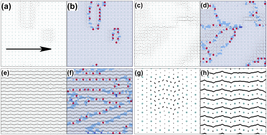
Figure 2: (Color online) (a,c,e) The pinning site locations (open circles) and particle trajectories (black lines) over a fixed interval of time for the system at f = 4.035. (a) Fd = 0.05, (c) Fd = 0.08, and (e) Fd = 0.2. (b,d,f) Pinning site locations (open circles), particle trajectories (black lines), and Voronoi construction (blue lines) for the same sample at (b) Fd = 0.05, (d) Fd = 0.08, and (f) Fd = 0.2. The Voronoi polygons are colored according to their number of sides: 4 (dark blue), 5 (light blue), 6 (white), and 7 (red). (a,b) The moving grain boundary state; (c,d) the fluctuating grain boundary state; and (e,f) the continuous flow regime. (g) A blowup of the particle positions and trajectories from (a) showing more clearly the the localized motion near a grain boundary. (h) The same for the system in (e), showing more clearly that there are two types of pinned particles: those trapped at the pinning sites, and those trapped in the interstitial regions.
Depinning of the grain boundaries is responsible for reducing the depinning force at the incommensurate fillings. Above depinning at these fillings, the grain boundaries move continuously but the particles only move about a lattice constant each time a grain boundary passes over them. Thus, the velocity of the grain boundary is higher than that of the individual particles. The particles spend most of their time pinned and are mobile only for brief periods of time when the grain boundary or soliton moves past. This process is illustrated in Fig. 2(a) where we plot the particle trajectories over a fixed time for a sample with f = 4.035 at Fd = 0.05. The particle motion is localized and correlated with the positions of the grain boundaries, as shown by the corresponding Voronoi construction in Fig. 2(b); motion occurs only where the grain boundaries are located, while regions without grain boundaries remain pinned. When the particles move, their trajectories are not strictly 1D but have a zig-zag shape since the particles must shift in both the x and y directions to permit the grain boundary to pass; the particles change from one triangular lattice orientation to the other after the grain boundary has moved over them. This motion has similarities to the soliton or kink motion observed near the f = 1.0 filling in experiments and simulations [40,21], but instead of isolated moving kinks or antikinks, we have a moving row of correlated kinks or antikinks that is bound to the grain boundary. The shape of the moving domain defined by the grain boundary does not remain completely static but can undergo expansions and contractions as it moves.
For Fd = 0.08, we find a transition from well-defined domain walls that move coherently across the system to a state where the domain walls break apart and reform, as illustrated in Fig. 2(c). The particle motion remains localized to the vicinity of the domain walls, as shown in Fig. 2(d). The number of domain walls strongly fluctuates in this state, which resembles the kink-antikink nucleation regime observed in the experiments of Ref. [40]. At Fd = 0.2, the flow of the mobile particles transitions from mostly static with small jumps every time a grain boundary passes to continuous motion. The immobile particles include the interstitially pinned particles as well as all of the directly pinned particles. The soliton motion is lost in this regime, as illustrated in Fig. 2(e), and the grain boundary state is destroyed due to a proliferation of 5-fold and 7-fold coordinated particles, as shown in Fig. 2(f). At f=3.965, where there is also a grain boundary pinned state, we find a sequence of dynamical states very similar to those shown in Fig. 2 for f = 4.035.
In order to more clearly illustrate the dynamics of the particles, in Fig. 2(g) we show the particle locations and trajectories from the system in Fig. 2(a) at Fd = 0.05 for a small region of the sample containing the grain boundary. Here, the particles move only near the grain boundary in a localized manner. In Fig. 2(h) we show the same type of plot for the system in Fig. 2(e) at Fd = 0.2 where there are two types of pinned particles, those pinned directly in the pinning sites and those pinned in the interstitial regions. The mobile particles form ordered winding channels similar to those that appear at f = 4.0. In the two stage depinning processes that occur at f = 4.035 and f=3.965, the grain boundaries depin first and there is only localized particle motion. This is followed by the depinning of channels of particles as shown in Fig. 2(h). As we further increase Fd, there are additional transitions to states with larger numbers of moving interstitial particles, while for sufficiently large Fd the directly pinned particles depin.
Fig3.png
Figure 3: (Color online) The velocity histograms for the system in Fig. 2 with f=4.035, averaged over ten realizations. (a,b,c) P(vx); (d,e,f) P(vy). (a,d) Fd = 0.05. (b,e) Fd = 0.12. (c,f) Fd = 0.2. Lines (black): increasing sweep of Fd. Bars (red): decreasing sweep of Fd.
We can identify four distinct dynamical regimes for the grain boundary forming fillings: (I) pinned; (II) grain boundary motion; (III) moving fluctuating grain boundaries; and (IV) continuous interstitial flow. The different regimes can also be characterized with the distributions P(vx) and P(vy) of the instantaneous particle velocities averaged over the ten realizations, as shown for the f = 4.035 sample at Fd = 0.05 in Fig. 3(a). Here, in the moving grain boundary state, there is a peak in P(vx) at vx = 0.0 from the immobile particles, a second peak near vx = 0.025, and continuous weight between the two peaks. Although the grain boundaries move at constant speed, the individual particles start with vx=0, reach a maximum velocity as the grain boundary moves past, and then drop back to the vx=0 state. As a result, we observe the full range of velocities between vx=0 and vx=0.025. Fig. 3(d) shows that the y velocities of the particles at the same drive are not strictly zero due to the zig-zag motion associated with the grain boundaries; however, the average value of vy is zero. For Fd = 0.12 in the same system, P(vx) in Fig. 3(b) extends to higher positive vx values than for the Fd=0.05 case, but the secondary peak in P(vx) disappears due to the strongly fluctuating nature of the grain boundary motion in this regime. In the corresponding P(vy) shown in Fig. 3(e), the tails have moved out further in the positive and negative vy directions.
For Fd = 0.20 in the continuous flow regime, P(vx) in Fig. 3(c) has two distinct peaks centered at vx = 0.0 and vx = 0.16. A region of zero weight exists between the two peaks, indicating that there are no particles moving at intermediate velocities. This is due to the loss of the soliton-like motion; in the continuous flow regime, the mobile particles always remain in motion while the pinned particles always remain immobile. The corresponding P(vy) in Fig. 3(f) is still centered at zero but now shows additional structure with two satellite peaks that arise due to the sinuous motion in this regime, illustrated in Fig. 2(e,h). For increasing Fd, P(vx) and P(vy) retain the same form shown in Fig. 3(c,f) until the particles at the pinning sites depin, upon which a new set of dynamical states appears that will not be considered in this work.
To test for hysteretic effects, we sweep Fd from Fd=0 up to Fd=0.35 and back down to Fd=0, then compare P(vx) and P(vy) obtained at the same value of Fd during the increasing and decreasing sweeps. In the continuous flow regime, Fig. 3(c) shows that there is no hysteresis; however, in the moving fluctuating grain boundary regime in Fig. 3(b), the system is generally more disordered during the decreasing Fd sweep, indicating that the fluctuating grain boundary regime persists down to a lower drive than that at which it first appeared during the upward sweep of Fd. Once the drive is low enough, the grain boundaries reform and the hysteresis is lost, as shown in Fig. 3(a).
For f = 3.965, a similar sequence of phases occur with similar characteristics in the velocity histograms; however, in this case the moving grain boundary regime persists up to higher drives before the moving fluctuating grain boundary regime appears. We find the same general features of the velocity histograms and dynamic phases for other fillings where grain boundary formation occurs in the pinned state, which are generally close to integer fillings such as near f = 3.0 and f = 4.0.

B.  Stripes and Symmetry Breaking Flows

Fig4.png
Figure 4: (Color online) The dynamics at f = 4.3, where the zero drive state forms a stripe pattern of topological defects. (a) The particle trajectories over time for the moving stripe state at Fd = 0.05. The particles do not move in the driving direction; instead, they translate in the positive x and negative y directions in the transverse flow state. (b) Voronoi construction (lines, blue) of the moving stripe state in (a). (c) The corresponding structure factor S(k) indicates that the system is ordered. (d) The particle trajectories over time for the disordered flow state at Fd=0.35, where the particles form 1D channels of flow in the direction of the drive. (e) Voronoi construction of the disordered flow state in (d). (f) The corresponding S(k) shows that the sample has a smectic type ordering. The Voronoi polygons are colored according to their number of sides: 4 (dark blue), 5 (light blue), 6 (white), and 7 (red).
At filling fractions where the topological defects form stripe structures, the system initially depins into a moving stripe phase, as shown in Fig. 4(b) for f = 4.3 and Fd = 0.05. The moving state is highly ordered, as indicated by the structure factor S(k) plotted in the inset of Fig. 4(c). At higher drives there is a transition to a state where the stripe structure breaks down and the system becomes more disordered, as shown in Fig. 4(e) for Fd = 0.35. In Fig. 4(f), the anisotropic features in S(k) reveal that the system is more disordered with smectic ordering along the x-direction.
In the moving stripe phase, the particles flow at an angle to the driving direction instead of along it, forming the transverse flow regime illustrated in Fig. 4(a) for the state in Fig. 4(b). Here the particles travel in both the positive x and negative y directions, while at Fd = 0.35, Fig. 4(d) indicates that the flow is now strictly in the x-direction. In the moving smectic phase at Fd = 0.35, the particles at the pinning sites and some of the interstitial particles are immobile, while the moving interstitial particles form channels of 1D flow. The number of particles can vary in each of the moving rows, causing most of the topological defects shown in Fig. 4(e) to align with the direction of drive and producing the ansiotropic or smectic type ordering shown in S(k) in Fig. 4(f). Smectic type flows of particles in periodic pinning array structures have been observed in simulations of vortices and colloidal particles moving over quasiperiodic arrays [44,42] as well as for the incommensurate flow in periodic arrays [49].
Fig5.png
Figure 5: (Color online) 〈Vx〉 vs Fd curves for increasing (lower center, black) and decreasing (upper center, red) sweeps of Fd at fillings that form pinned stripe states. (a) At f = 4.3, there is a jump up in 〈Vx 〉 near Fd = 0.1 at the transition from stripe flow to smectic flow. Inset: the corresponding 〈Vy〉 vs Fd shows that in the stripe flow regime, the particles are also flowing in the negative y-direction, but this motion is lost at the stripe-smectic flow transition, which is hysteretic. (b) 〈Vx〉 vs Fd for f = 3.7. Here the smectic flow is stable all the way down to Fd = 0. Inset: The corresponding 〈Vy〉 vs Fd.
The symmetry breaking flow produces signatures in the velocity force curves 〈Vx〉 vs Fd, as shown in Fig. 5(a,b) for two states that form pinned periodic stripes, f = 4.3 and f=3.7. Here the black line is for the initial upward sweep of Fd, and the red line is for sweeping Fd back down to zero. Neither of these fillings have a finite depinning threshold within our resolution; however, both have a two-step velocity response, which for f = 4.3 in Fig. 5(a) is associated with a jump up in 〈Vx〉 just above Fd = 0.1. In the inset of Fig. 5(a) we plot the corresponding 〈Vy〉 vs Fd, where we find a linear increase in the negative y-direction velocity followed by a sharp jump into a fluctuating state with 〈Vy〉 = 0 at the same value of Fd where a jump in 〈Vx〉 appears in the main panel. This feature marks the transition from symmetry breaking flow of stripes to the 1D winding smectic flow. The velocity-force curves in Fig. 5(a) and its inset also show hysteresis across the stripe-smectic flow boundary, indicating that when the external drive is reversed, the system can remain in the smectic flow state down to a drive lower than that at which the state first appeared during the increasing sweep of Fd. For f = 3.7, Fig. 5(b) shows that a similar set of dynamics occurs; however, in this case the smectic flow persists for the decreasing sweep of Fd all the way down to Fd = 0. In general, we observe symmetry breaking flow in regimes where stripe domain wall patterns form. Symmetry breaking flows have also been found for driven vortex systems when the vortices form effective composite objects such as dimers that possess an orientational degree of freedom [53]. This is different from the present situation, where the symmetry breaking is a result of the large scale symmetric patterns that form. Symmetry breaking flow has also been observed in simulations of colloidal particles moving over egg-carton arrays in the weak substrate limit when the particles form a triangular lattice that does not have the same orientation as the substrate lattice [20]. In that case the entire lattice flows elastically. This differs from the flow shown in Fig. 4, where the motion is confined only to the grain boundaries and does not involve all the particles in the system.
Fig6.png
Figure 6: (Color online) The velocity histograms for f = 4.3. (a,b,c) P(vx); (d,e,f) P(vy). (a,d) Fd = 0.05. (b,e) Fd = 0.1. (c,e) Fd = 0.35. Lines (black): Increasing sweep of Fd. Filled curves (red): Decreasing sweep of Fd.
In Fig. 6(a,d) we show the velocity histograms at f = 4.3 and Fd = 0.05. Here P(vx) has a positive average value with several peaks, while the corresponding P(vy) has a net negative value due to the symmetry breaking flow along the negative y-direction. The peaks arise because the particles move in a synchronized highly ordered flow, producing a periodic velocity time series. For Fd = 0.10 in Fig. 6(b,e), stripe flow occurs for the initial ramp up of the external drive; however, during the ramp down, the system remains in a smectic flow regime so that 〈Vy〉 = 0, as shown by the symmetric P(vy) in Fig. 6(e). At Fd = 0.35 in the smectic flow regime, P(vx) in Fig. 6(c) has two prominent peaks, but the additional smaller scale peaks that appeared for the symmetry breaking flow are lost when the different channels move at different velocities, producing a disordered flow that smears the velocity distributions. The corresponding P(vy) has a symmetric profile, indicating that the flow is oriented in the x-direction. The two satellite peaks in P(vy) are due to the semi-periodic oscillations of a number of the channels, as shown in the trajectory images in Fig. 4(d). We observe a similar set of velocity distributions at f = 3.7 as well as at other fillings where the stripe state appears. At f = 4.5, the static phase does not form stripes but instead organizes into a checkerboard pattern [4]. When this pattern is driven, it transforms into a stripe phase and undergoes dynamics similar to those described for the f=4.3 system.


IV.  FLOW FROM 4.6 < f ≤ 5.0

Fig7.png
Figure 7: (Color online) (a) 〈Vx〉 vs Fd for a filling of f = 4.7 (upper right, black) and f = 5.0 (lower right, purple). (b) The corresponding P6 vs Fd.
Fig8.png
Figure 8: The particle trajectories in a portion of the sample over a fixed time interval for the f = 4.7 state. (a) Fd = 0.05 (b) Fd = 0.1, (c) Fd = 0.2 and (d) Fd = 0.35.
In the range 4.6 < f < 5.0, the static ordered stripe states are replaced by disordered patch regimes. The patches consist of regions of square ordering that grow in extent with increasing f until the entire system forms a square lattice at f=5.0. [4] The depinning threshold is finite in the patch regime; however, the velocity response is smooth, as shown in Fig. 7(a) where we plot 〈Vx〉 vs Fd for f = 4.7. At f = 5.0, Fig. 7(a) shows that there is a sharp finite depinning threshold, while at f = 4.7 the depinning threshold drops to Fd = 0.025 and the response above depinning increases smoothly. Above depinning for f = 4.7, shown in Fig. 8(a) for Fd=0.05, disordered winding channels of flow form that are composed of localized soliton type pulses randomly distributed throughout the system. At Fd = 0.1, shown in Fig. 8(b), these disordered flow regions start to proliferate. At the higher drive Fd = 0.2, illustrated in Fig. 8(c), the flow is more strongly disordered, while at Fd = 0.35, shown in Fig. 8(d), the flow starts to become more ordered and is confined into 1D winding channels in the interstitial regions. Figure 7(b) shows that P6 vs Fd for f = 4.7 undergoes very little change over the range of drives examined. In contrast, for f = 5.0, P6 starts at zero since the system exhibits square ordering. As Fd increases, the system disorders, causing a jump in P6 below the depinning threshold. For higher drives P6 reaches a steady state value. For fillings above f = 5.0, the depinning threshold decreases and there is a two stage depinning response.
At f = 4.7, there is no hysteresis in the response to a drive. The velocity force characteristics for f = 4.7 in Fig. 7(a) can be fit to the power-law form V ∝ (FdFc)β, where Fc is the critical depinning force. We find 1.5 < β < 2.0, consistent with the values obtained for disordered flows in the depinning of colloidal systems driven over random substrates [50] and for vortices driven over random pinning [51]. This indicates that although the system has an underlying periodic substrate, there are certain fillings where the strong structural disorder caused by frustration effects can produce dynamics that resemble those found for systems with random substrates.
Fig9.png
Figure 9: (Color online) The velocity histograms P(vx) for f = 4.7 at Fd = 0.05 (red), 0.1 (green), 0.2 (blue), and 0.35 (purple), from lower right to upper right.
Fig10.png
Figure 10: (Color online) A schematic dynamic phase diagram for Fd vs f in the range 4.0 ≤ f ≤ 5.0 indicating the pinned phase P, the continuous flow phase C, the disordered flow phase D, the transverse flow phase T, and the grain boundary flow phase GB. The dashed line inside the GB phase indicates the separation between coherent (below line) and incoherent (above line) grain boundary flow.
The velocity histograms P(vx) at f = 4.7 plotted in Fig. 9 for different values of Fd show that there is no gap between the zero velocity peak and the higher velocity peak in the disordered flow regime, even at the higher drive of Fd = 0.35, although the peak at higher vx becomes strongly smeared. Simulations of vortices moving over random substrates produced a series of velocity histograms for increasing drive with similar characteristics [52]. For the filling at f = 4.7, the initial motion near Fd = 0.05 has a soliton or crinkle type form where pulses move through the system and individual particles move only about a lattice constant each time the pulse passes by. Unlike what we observe at more ordered fillings, here the pulse motion is not strictly confined to 1D but can show considerable transverse mobility as well. The system gradually transitions to a state with a combination of soliton type motion and continuous motion near Fd = 0.2, while at Fd = 0.35 the motion is mostly continuous.
In order to better illustrate the different dynamic phases, in Fig. 10 we present a schematic dynamical phase diagram of Fd versus f in the regime 4.0 ≤ f ≤ 5.0. Here, peaks in Fc occur at the ordered fillings of f = 4.0, 4.5, and 5.0. The transverse flow appears only for 4.1 < f < 4.5, while grain boundary flow occurs for 4 < f < 4.1, with the dashed line representing the crossover from coherent to incoherent grain boundary flow. For 4.5 < f < 5.0, the system depins into a disordered flow state.


V.  FLOW NEAR f = 3.0 and 2.0

Fig11.png
Figure 11: (Color online) (a) 〈Vx〉 vs Fd for f = 3.0 (highest depinning threshold, black), f = 2.9 (middle depinning threshold, purple), and f = 3.1 (lowest depinning threshold, green). (b) P4 (center left, dark blue), P5 (upper right, light blue), P6 (lower left, gray), and P7 (upper left, red) vs Fd for the f = 3.0 case.
Fig12.png
Figure 12: (Color online) (a) The Voronoi construction (lines, blue) for the f = 3.0 pinned state in a portion of the sample. The Voronoi polygons are colored according to their number of sides: 4 (dark blue) and 7 (red). (b) The corresponding particle (dot) and pinning site (circle) locations showing the effective dimerization of the two interstitial particles per pinning site plaquette.
For fillings of 2.9 < f < 3.0 and 3.0 < f < 3.1, the system forms grain boundaries and exhibits dynamics similar to those of the grain boundary forming states near f = 4.0. In Fig. 11(a) we plot 〈Vx〉 vs Fd for f = 2.9, 3.0, and 3.1. Here the maximum in the depinning threshold Fc occurs for f = 3.0 near Fd = 0.125, with a lower Fc for f=2.9 and an even lower Fc for f=3.1. In all cases there is a multiple step depinning process, and the initial motion for f = 3.1 and f=2.9 occurs via the depinning of the grain boundaries. In Fig. 11(b) we plot P4, P5, P6, and P7 for the f = 3.0 state. Here, in the ordered ground state lattice the two interstitial particles in each pinning plaquette form an effective dimer that can be oriented either vertically or horizontally, as illustrated in Fig. 12. Just above Fd = 0.125, depinning occurs and is accompanied by a small jump in Pn, with n=4, 5, 6, 7.
Fig13.png
Figure 13: (Color online) (a) 〈Vx〉 vs Fd for f = 2.0 (highest depinning threshold, black) f = 1.95 (middle depinning threshold, purple), and f = 2.05 (lowest depinning threshold, green). (b) The corresponding P4 vs Fd. (c) The corresponding P6 vs Fd.
At f = 2.0 the system forms a square lattice, while at f = 1.95 and f = 2.05 the incommensurate configurations do not form grain boundaries but instead contain isolated islands similar to those found at the fillings 0.9 < f < 1.0 and 1.0 < f < 1.1. In Fig. 13(a) we plot Vx vs Fd for f=1.95, 2.0, and 2.05. The highest depinning threshold occurs for f = 2.0, where the depinning occurs via the continuous flow of the interstitial particles while the particles at the pinning sites remain pinned. At drives higher than those shown in the figure, a second depinning transition occurs when the particles at the pinning sites become mobile. At f = 2.05, the interstitial depinning occurs in two steps. Above the first step, we find soliton type motion of the extra interstitial particles in the square lattice ground state, while above the second step we find the same type of depinning that occurs at f=2.0 where all the interstitial particles move. For f = 1.95, a similar scenario occurs; however, the depinning threshold is higher than for f=2.05 since for f=1.95 the initial depinning is of vacancies or antikinks which have a higher depinning threshold than the kinks. In Fig. 13(b,c) we plot P4 and P6, respectively, versus Fd for the same three fillings. At f=2.0 the system depins into a disordered flowing state. A similar trend occurs for the incommensurate cases with additional disorder.


VI.  DISCUSSION

We have shown that numerous dynamical transitions can occur in this system, and it is interesting to ask how these transitions relate to the static annealed states studied previously in Ref. [4]. It is possible that the system becomes trapped in a metastable state during the annealing process rather than reaching a true lowest energy state. Application of a driving force could overcome the kinetic barriers holding the system in the metastable state and allow it to access a lower energy state. We have performed a series of studies with different annealing rates and find that for rates slower than those considered here, the type of patterns that form remain the same, indicating that we are not quenching our system. Under a driving force, the fluctuations experienced by the particles are not of Boltzmann type, as indicated by the velocity histograms. In addition, the number of high-energy dislocations in the system typically increases in the driven state, so that the configuration energy generally increases rather than decreasing under driving. In certain spin systems, it is known that cycling an external field can cause the system to hysteretically approach a lower energy state. In our system, the transitions between the different dynamical states are generally sharp, suggesting that they are first order in nature. As a result, partially disordered phases that are created when ramping up an external drive can persist to much lower drives when the driving force is ramped back down, and since the velocity fluctuations in the driven state are dynamical rather than thermal, these states cannot simply anneal away. We find that the hysteresis during the first driving cycle is the largest, and then reaches a steady state width in successive cycles.
In this work we focus on driving in the x-direction. If the driving is applied along the y-direction, we find essentially the same behavior in the grain boundary and defect states; however, some differences emerge in the stripe states. For example, if the system in Fig. 4 is driven in the y direction, just above depinning the particles move in the positive y and positive x directions, while for higher drives the motion is strictly in the positive y direction. The transverse stripe flow phases appear for driving in either the x or y direction. It is also possible to apply the drive at an arbitrary angle with respect to the underlying square pinning substrate. Previous work on particles driven over square pinning arrays at different drive angles for fillings close to f=1 showed that a rich variety of driven phases occur in conjunction with dynamical locking, where the flow locks to certain angles of the form θ = arctan(Fy/Fx) due to the square symmetry [54]. At the higher fillings we consider here, we expect that a number of new dynamical phenomena could arise if the drive angle were continuously rotated, but these are beyond the scope of the present work.
Finally, we compare the colloidal particle system studied here with other related systems in which similar behavior could occur. For example, for vortices in type-II superconductors with periodic arrays of artificial pinning sites that are small enough to capture only a single vortex each, the same static states found in Ref. [4] have been observed experimentally for f=2.0, 3.0, and 4.0 [5]. These vortex imaging experiments could access only relatively small regions of space, and vortex arrangements at incommensurate fillings were never studied [7]. Under an applied drive, a number of incommensuration and soliton vortex flow states were observed at fillings few percent above and below f = 1.0 [8]. Simulations at high fillings in these vortex systems produced a variety of dynamical phases [62]; however, experimental observations of these regimes have proven difficult, in part due to the possibility of multiply occupied pinning sites. Since the vortices have no hard core, they can merge to form multiquantized vortex states trapped at the pinning sites. In addition, most superconducting samples contain intrinsic random pinning that can be strong enough to disrupt grain boundary flows of the type we consider here. In colloidal systems such intrinsic pinning does not exist. In frictional systems where there is one atomic layer adsorbed on an atomic or molecular surface, the filling fractions are generally limited to values close to the first filling.
In this work we restrict ourselves to particles with only isotropic repulsive interactions; however, there are many examples of systems with competing interactions such as particles with short range attraction and long range repulsion [56,57,59] or particles with short range repulsion and intermediate range attraction [55]. In such systems, a variety of crystalline and partially ordered states, including stripe, clump, bubble, and crystalline phases [58,57], can form in the absence of any substrate. When a substrate is added, it may be possible to realize stripe states for fillings close to f=1. It would be interesting to understand whether dynamics similar to those we observe for the grain boundary and stripe states are general to such pattern forming systems.
There has also been work on a 2D system of particles in which a square phase can be stabilized in the absence of a substrate due to a three-body interaction term [61,60]. A rich variety of phases appear in this system, and when the particles are driven over a random substrate, it is possible to have coexisting dynamical phases similar to the phase coexistence observed in equilibrium systems. It would be interesting to study both the equilibrium and dynamical properties of this system in the presence of periodic substrates. Refs. [60,61] showed that an effective shaking temperature can be measured in the driven state. The shaking temperature concept was originally developed in Ref. [63] for particles moving over a random substrate where, even at zero thermal temperature, the particles experience fluctuations due to their motion over the substrate. These fluctuations can be described in terms of an effective temperature called the shaking temperature. As the drive increases, the effectiveness of the substrate decreases and the shaking temperature decreases as Tsh ∝ 1/vcm, where vcm is the center of mass velocity. In Refs. [60,61], some of the dynamical phases could be well fit to a shaking temperature, while others had distinct changes in the shaking temperatures associated with the dynamics of different phases. Attempting to perform a shaking temperature analysis for our system is problematic since our substrate is periodic rather than random, and many of the dynamic phases are strongly crystalline and lack fluctuations of thermal character. In the disordered flow regime, such an analysis could probably be done but is beyond the scope of the present work.


VII.  SUMMARY

We have investigated the sliding dynamics for colloidal particles on periodic two dimensional muffin-tin type pinning arrays. In the static case this system was previously shown to exhibit pattern formation in the form of domain walls, stripes, and disordered phases at incommensurate fillings, particularly in the range 4.0 < f < 5.0. Here we find that a rich variety of distinct dynamical phases occur in this system including domain wall dynamics as well as disordered and continuous flow phases associated with characteristic velocity distributions and structural order. Transitions between dynamic phases produce distinct features in the velocity force curves, velocity histograms, particle trajectories, and structural ordering. The system is most strongly pinned at the commensurate fillings, while at the incommensurate fillings it is weakly pinned and undergoes multiple depinning transitions. The initial depinning occurs via soliton type motion or by the motion of domain walls. In the domain wall regime, when the domain wall depins, individual particles only move about a lattice constant each time the domain wall moves past. For increasing drive the domain walls start to fluctuate, and at higher drives there is a transition to the continuous flow of interstitial particles when the domain wall structure breaks apart. In the regime where the domain walls form stripes, the particles move at an angle with respect to the drive above depinning, while at higher drives the stripes break apart and the particle motion is in the direction of drive. For fillings 4.6 < f < 5.0, the domain wall structure is replaced with disordered patches, and for increasing drive we only observe disordered flow. For 2.9 < f < 3.0 and 3.0 < f < 3.1, we find a multi-step depinning of domain walls, while at 1.9 < f < 2.0, instead of domain walls we observe individual interstitial and vacancy particles that depin first followed by the continuous flow of all or a portion of the interstitial particles at higher drives. Our results on how the motion of domain walls or incommensurations leads to different dynamical responses should be general to other systems exhibiting commensurate-incommensurate transitions, such as friction on incommensurate surfaces where domain walls are present or the flow of vortices in type-II superconductors.
This work was carried out under the auspices of the NNSA of the U.S. DoE at LANL under Contract No. DE-AC52-06NA25396. D.M. and J.A. received support from the ASC Summer Workshop program at LANL.

References

[1]
P. Bak, Rep. Prog. Phys. 45, 587 (1982).
[2]
S.N. Coppersmith, D.S. Fisher, B.I. Halperin, P.A. Lee, and W.F. Brinkman, Phys. Rev. Lett. 46, 549 (1981).
[3]
S. Bleil, H.H. von Grünberg, J Dobnikar, R. Castañeda-Priego and C Bechinger, Europhys. Lett. 73, 450 (2006).
[4]
D. McDermott, J. Amelang, L.M. Lopatina, C.J. Olson Reichhardt, and C. Reichhardt, Soft Matter 9, 4607 (2013).
[5]
K. Harada, O. Kamimura, H. Kasai, T. Matsuda, A. Tonomura, and V.V. Moshchalkov, Science 274, 1167 (1996).
[6]
C. Reichhardt, J. Groth, C.J. Olson, S.B. Field, and F. Nori, Phys. Rev. B 54, 16108 (1996).
[7]
C. Reichhardt, C.J. Olson, and F. Nori, Phys. Rev. B 57, 7937 (1998).
[8]
J. Gutierrez, A.V. Silhanek, J. Van de Vondel, W. Gillijns, and V.V. Moshchalkov, Phys. Rev. B 80, 140514 (2009).
[9]
W.V. Pogosov, H.J. Zhao, V.R. Misko, and F.M. Peeters, Phys. Rev. B 81, 024513 (2010).
[10]
S. Avci, Z.L. Xiao, J. Hua, A. Imre, R. Divan, J. Pearson, U. Welp, W.K. Kwok, and G.W. Crabtree, Appl. Phys. Lett. 97, 042511 (2010).
[11]
S. Tung, V. Schweikhard, and E.A. Cornell, Phys. Rev. Lett. 97, 240402 (2006); H. Pu, L.O. Baksmaty, S. Yi, and N.P. Bigelow, Phys. Rev. Lett. 94, 190401 (2005).
[12]
G. Grüner, Rev. Mod. Phys. 60, 1129 (1988).
[13]
J. Chakrabarti, H. R. Krishnamurthy, A. K. Sood, and S. Sengupta, Phys. Rev. Lett. 75, 2232 (1995); Q.-H. Wei, C. Bechinger, D. Rudhardt, and P. Leiderer, Phys. Rev. Lett. 81, 2606 (1998); C. Das, A. K. Sood, and H. R. Krishnamurthy, Physica A 270, 237 (1999); W. Strepp, S. Sengupta, and P. Nielaba, Phys. Rev. E 63, 046106 (2001) D. Chaudhuri and S. Sengupta, Europhys. Lett. 67, 814 (2004); C. Bechinger, M. Brunner, and P. Leiderer, Phys. Rev. Lett. 86, 930 (2001); C. Mondal and S. Sengupta, Phys. Rev. E x, 020402 (2012).
[14]
C. Reichhardt and C.J. Olson, Phys. Rev. Lett. 88, 248301 (2002).
[15]
M. Brunner and C. Bechinger, Phys. Rev. Lett. 88, 248302 (2002).
[16]
A. Libál, C. Reichhardt, and C.J. Olson Reichhardt, Phys. Rev. Lett. 97, 228302 (2006).
[17]
A. Sarlah, E. Frey, and T. Franosch, Phys. Rev. E 75, 021402 (2007).
[18]
S. El Shawish, J. Dobnikar, and E. Trizac, Soft Matter 4, 1491 (2008).
[19]
C. Reichhardt and C. J. Olson Reichhardt Phys. Rev. E 80, 022401 (2009).
[20]
C. Reichhardt and C.J. Olson Reichhardt, Phys. Rev. E 85, 051401 (2012).
[21]
A. Vanossi, N. Manini, and E. Tosatti, Proc. Natl. Acad. Sci. 109, 16429 (2012).
[22]
P. Tierno, Soft Matter 8, 11443 (2012).
[23]
G. Coupier, M. Saint Jean, and C. Guthmann, Phys. Rev. B 75, 224103 (2007).
[24]
O.M. Braun, T. Dauxois, M.V. Paliy, and M. Peyrard, Phys. Rev. Lett. 78, 1295 (1997).
[25]
O.M. Braun, T. Dauxois, M.V. Paliy, and M. Peyrard, Phys. Rev. E 55, 3598 (1997).
[26]
O.M. Braun, M.V. Paliy, J. Röder, and A.R. Bishop, Phys. Rev. E 63, 036129 (2001).
[27]
O.M. Braun and Y.S. Kivshar, The Frenkel-Kontorova Model: Concepts, Methods, and Applications (Springer, 2004).
[28]
C.V. Achim, J.A.P. Ramos, M. Karttunen, K.R. Elder, E. Granato, T. Ala-Nissila, and S.C. Ying, Phys. Rev. E 79, 011606 (2009).
[29]
Y. Yang, W.-S. Duan, J.-M. Chen, L. Yang, J. Tekic, Z.-G. Shao, and C.-L. Wang, Phys. Rev. E 82, 051119 (2010).
[30]
A. Benassi, A. Vanossi, and E. Tosatti, Nature Commun. 2, 236 (2011).
[31]
A. Vanossi, N. Manini, M. Urbakh, S. Zapperi, and E. Tosatti, Rev. Mod. Phys. 85, 529 (2013).
[32]
A. Chowdhury, B.J. Ackerson, and N.A. Clark, Phys. Rev. Lett. 55, 833 (1985).
[33]
P. Tierno, Phys. Rev. Lett. 109, 198304 (2012).
[34]
P.T. Korda, M.B. Taylor, and D.G. Grier, Phys. Rev. Lett. 89, 128301 (2002).
[35]
M.A. Tahir, L. Gao, L.N. Virgin, and B.B. Yellen, Phys. Rev. E 84, 011403 (2011).
[36]
M. Balvin, E. Sohn, T. Iracki, G. Drazer, and J. Frechette, Phys. Rev. Lett. 103, 078301 (2009).
[37]
T. Neuhaus, M. Marechal, M. Schmiedeberg, and H. Löwen, Phys. Rev. Lett. 110, 118301 (2013).
[38]
J. Hasnain, S. Jungblut, and C. Dellago, Soft Matter 9, 5867 (2013).
[39]
A. Pertsinidis and X.S. Ling, Phys. Rev. Lett. 100, 028303 (2008).
[40]
T. Bohlein, J. Mikhael, and C. Bechinger, Nature Mater. 11, 126 (2011).
[41]
M. Peyard and S.J. Aubry, J. Phys. C 16, 1593 (1983).
[42]
C. Reichhardt and C. J. Olson Reichhardt, Phys. Rev. Lett. 106, 060603 (2011).
[43]
J.A. Kromer, M. Schmiedeberg, J. Roth, and H. Stark, Phys. Rev. Lett. 108, 218301 (2012).
[44]
T. Bohlein and C. Bechinger, Phys. Rev. Lett. 109, 058301 (2012).
[45]
J. Mikhael, J. Roth, L. Helden, and C. Bechinger, Nature 454, 501 (2008).
[46]
M. Schmiedeberg and H. Stark, Phys. Rev. Lett. 101, 218302 (2008).
[47]
C. Reichhardt, C.J. Olson, and F. Nori, Phys. Rev. Lett. 78, 2648 (1997).
[48]
K. Mangold, P. Leiderer, and C. Bechinger, Phys. Rev. Lett. 90, 158302 (2003).
[49]
C. Reichhardt and C.J. Olson Reichhardt, J. Phys.: Condens. Matter 24, 225702 (2012).
[50]
K. Nelissen, B. Partoens, and F. M. Peeters, Phys. Rev. E 71, 066204 (2005); C. Reichhardt and C.J. Olson, Phys. Rev. Lett. 89, 078301 (2002).
[51]
S. Bhattacharya and M.J. Higgins, Phys. Rev. Lett. 70, 2617 (1993); D. Domínguez, Phys. Rev. Lett. 72, 3096 (1994).
[52]
M.C. Faleski, M.C. Marchetti, and A.A. Middleton, Phys. Rev. B 54, 12427 (1996).
[53]
C. Reichhardt and C. J. Olson Reichhardt, Phys. Rev. B 78, 224511 (2008).
[54]
C. Reichhardt and F. Nori, Phys. Rev. Lett. 82, 414 (1999); P T. Korda, M.B. Taylor, and D.G. Grier, Phys. Rev. Lett. 89, 128301 (2002).
[55]
M. Golosovsky, Y. Saado, and D. Davidov, Phys. Rev. E 65, 061405 (2002); H.J. Zhao, V.R. Misko, and F.M. Peeters, New J. Phys. 14, 063032 (2012).
[56]
C. J. Olson Reichhardt, C. Reichhardt, I. Martin, and A. R. Bishop, Physica D 193, 303 (2004).
[57]
C.J. Olson Reichhardt, C. Reichhardt, and A. R. Bishop, Phys. Rev. E 82, 041502 (2010).
[58]
G. Malescio and G. Pellicane, Nature Mater. 2, 97 (2003); Phys. Rev. E 70, 021202 (2004); M.A. Glaser, G.M. Grason, R.D. Kamien, A. Kosmrlj, C.D. Santangelo, and P. Ziherl, EPL 78, 46004 (2007).
[59]
K. Nelissen, B. Partoens, and F. M. Peeters, Phys. Rev. E 71, 066204 (2005).
[60]
A. Sengupta, S. Sengupta, and G.I. Menon, Phys. Rev. B 81, 144521 (2010).
[61]
A. Sengupta, S. Sengupta, and G.I. Menon, Phys. Rev. B 75, 180201 (2007).
[62]
C. Reichhardt, G.T. Zimányi, and N. Grønbech-Jensen, Phys. Rev. B 64, 014501 (2001); C. Reichhardt and C.J. Olson Reichhardt, Phys. Rev. B 78, 224511 (2008).
[63]
A.E. Koshelev and V.M. Vinokur, Phys. Rev. Lett. 73, 3580 (1994).


File translated from TEX by TTHgold, version 4.00.

Back to Home