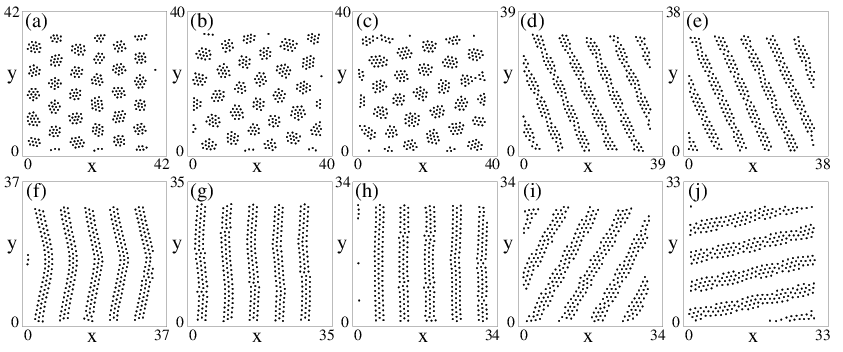
 Figure 3:
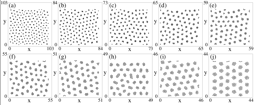
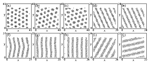
Particle locations in the entire sample after simulated annealing
for different densities in the clump and stripe regimes.
The scale of the x and y axes is not fixed in all panels.
(a)
ρ = 0.24, (b) ρ = 0.26, (c) ρ = 0.27, (d) ρ = 0.28,
(e) ρ = 0.30, (f) ρ = 0.32, (g) ρ = 0.34, (h) ρ = 0.36,
(i) ρ = 0.38, and (j) ρ = 0.40.
The clump phase appears for ρ < 0.28.
For 0.20 ≤ ρ < 0.28, the clumps form a triangular lattice.
For
0.28 ≤ ρ ≤ 0.44 a stripe phase occurs.
The stripe structures have some density modulations along their length for
ρ = 0.28 in panel (d) and ρ = 0.30 in panel (f),
but are more uniform for the higher densities. The stripe phases
at 0.32 ≤ ρ ≤ 0.36 in panels (f), (g), and (h)
contain three rows of particles per stripe.
Figure 3:
Particle locations in the entire sample after simulated annealing
for different densities in the clump and stripe regimes.
The scale of the x and y axes is not fixed in all panels.
(a)
ρ = 0.24, (b) ρ = 0.26, (c) ρ = 0.27, (d) ρ = 0.28,
(e) ρ = 0.30, (f) ρ = 0.32, (g) ρ = 0.34, (h) ρ = 0.36,
(i) ρ = 0.38, and (j) ρ = 0.40.
The clump phase appears for ρ < 0.28.
For 0.20 ≤ ρ < 0.28, the clumps form a triangular lattice.
For
0.28 ≤ ρ ≤ 0.44 a stripe phase occurs.
The stripe structures have some density modulations along their length for
ρ = 0.28 in panel (d) and ρ = 0.30 in panel (f),
but are more uniform for the higher densities. The stripe phases
at 0.32 ≤ ρ ≤ 0.36 in panels (f), (g), and (h)
contain three rows of particles per stripe.
|