Soft Matter 9, 4607 (2013)

Domain and Stripe Formation Between Hexagonal and Square Ordered Fillings of Colloidal Particles on Periodic Pinning Substrates

Danielle McDermott,^a,b Jeff Amelang,^a,c, Lena M. Lopatina,^a, Cynthia J. Olson Reichhardt,^∗^a and Charles Reichhardt^a

^aTheoretical Division, Los Alamos National Laboratory, Los Alamos, New Mexico 87545, USA. E-mail: cjrx@lanl.gov; Fax: +1 505 606 0917; Tel: +1 505 665 1134
^bDepartment of Physics, University of Notre Dame, Notre Dame, Indiana 46556, USA
^cDivision of Engineering and Applied Science, California Institute of Technology, Pasadena, California 91125, USA

Received 16th November 2012
Accepted 22nd January 2013

DOI: 10.1039/c3sm27652j

www.rsc.org/softmatter

Using large scale numerical simulations, we examine the ordering of colloidal particles on square periodic two-dimensional muffin-tin substrates consisting of a flat surface with localized pinning sites. We show that when there are four particles per pinning site, the particles adopt a hexagonal ordering, while for five particles per pinning site, a square ordering appears. For fillings between four and five particles per pinning site, we identify a rich variety of distinct ordering regimes, including disordered grain boundaries, crystalline stripe structures, superlattice orderings, and disordered patchy arrangements. We characterize the different regimes using Voronoi analysis, energy dispersion, and ordering of the domains. We show that many of the boundary formation features we observe occur for a wide range of other fillings. Our results demonstrate that grain boundary tailoring can be achieved with muffin-tin periodic pinning substrates.

1 Introduction
2 Simulation and System
3 Colloidal Particle Configurations
4 Analysis
5 Other fillings
6 Conclusions
References

1 Introduction

There is tremendous interest in understanding how to create different types of self-assembled colloidal structures. It would be particularly useful to identify methods for controlling domain formation and morphology. In two-dimensional systems of colloidal particles interacting with a repulsive Yukawa potential, the lowest energy configuration is a hexagonal lattice [1], but this ordering can be modified if the particles interact with a substrate potential. For random substrates, dislocations appear in the colloidal lattice and destroy the hexagonal ordering [2,3,4]. For periodic substrates, the hexagonal ordering may persist, but it is also possible for different ordered states as well as frustrated partially-ordered states to arise due to the competition between the colloidal interactions and the substrate.

For one-dimensional periodic substrates, triangular and smectic type orderings have been observed [5,6,7,8,9]. For two dimensional periodic substrates, the type of ordering depends on whether the number of colloidal particles is greater or less than the number of potential minima. In the case of egg-carton substrates, colloidal molecular crystal states appear whenever the number of colloidal particles per potential minima or the filling factor f is an integer with f=2 or higher. Here, the n particles in each potential trap form an n-mer state with an orientational degree of freedom, and this system can be mapped to various spin models [10,11,13,12,14]. Another type of two-dimensional substrate that has been experimentally realized is a muffin tin where the potential minima or pinning sites are defined as localized trapping sites of radius R_s surrounded by a flat region [15,16,17]. Experimental realizations of this system show that in this case there are two types of colloidal particle species: the particles that are directly trapped at the pinning sites, and the remaining particles that are localized on the flat part of the potential due to their interaction with the directly trapped particles. These are termed interstitially pinned particles, and they are much more mobile than the particles in an egg-carton potential [15]. Muffin tin-type potentials have been studied for the ordering and pinning of vortices in type-II superconductors, where different types of vortex crystalline states were shown to occur at integer fillings [18,19,20].

At noninteger incommensurate fillings, the system may become disordered. For colloidal particles in egg-carton potentials at fillings below the f=1 matching filling, certain crystalline type structures appear at rational fractional filling ratios such as f=1/3, while at other fillings, the system is either disordered or else domain wall structures form [21]. The ordering of repulsive particles for fillings less than one has been studied for vortices in Josephson junction arrays and in periodic pinning, where ordered and quasi-ordered patterns arise [22,23,24,20]. Such structures also have many strong similarities to atomic ordering on periodic substrates where the atomic coverage is less than a monolayer [25,26]. The incommensurate structures for colloidal particles on muffin type structures at higher filling fractions is not known; the additional degrees of freedom in the interstitial regions could allow for novel orderings or grain boundary structures that cannot form at incommensurate fillings on egg-carton potentials.

Here we show that colloidal particles at noninteger fillings on muffin tin potentials exhibit a remarkable variety of orderings, including a stripe crystalline regime dominated by fivefold and sevenfold coordinated particles. We also find other structures including grain boundaries, superlattices, and disordered patchy regimes. We specifically focus on fillings between four and five particles per trap; however, our results can be generalized to many other non-integer fillings with more than three particles per trap, and indicate that distinct grain boundary morphologies are a generic feature of this system.

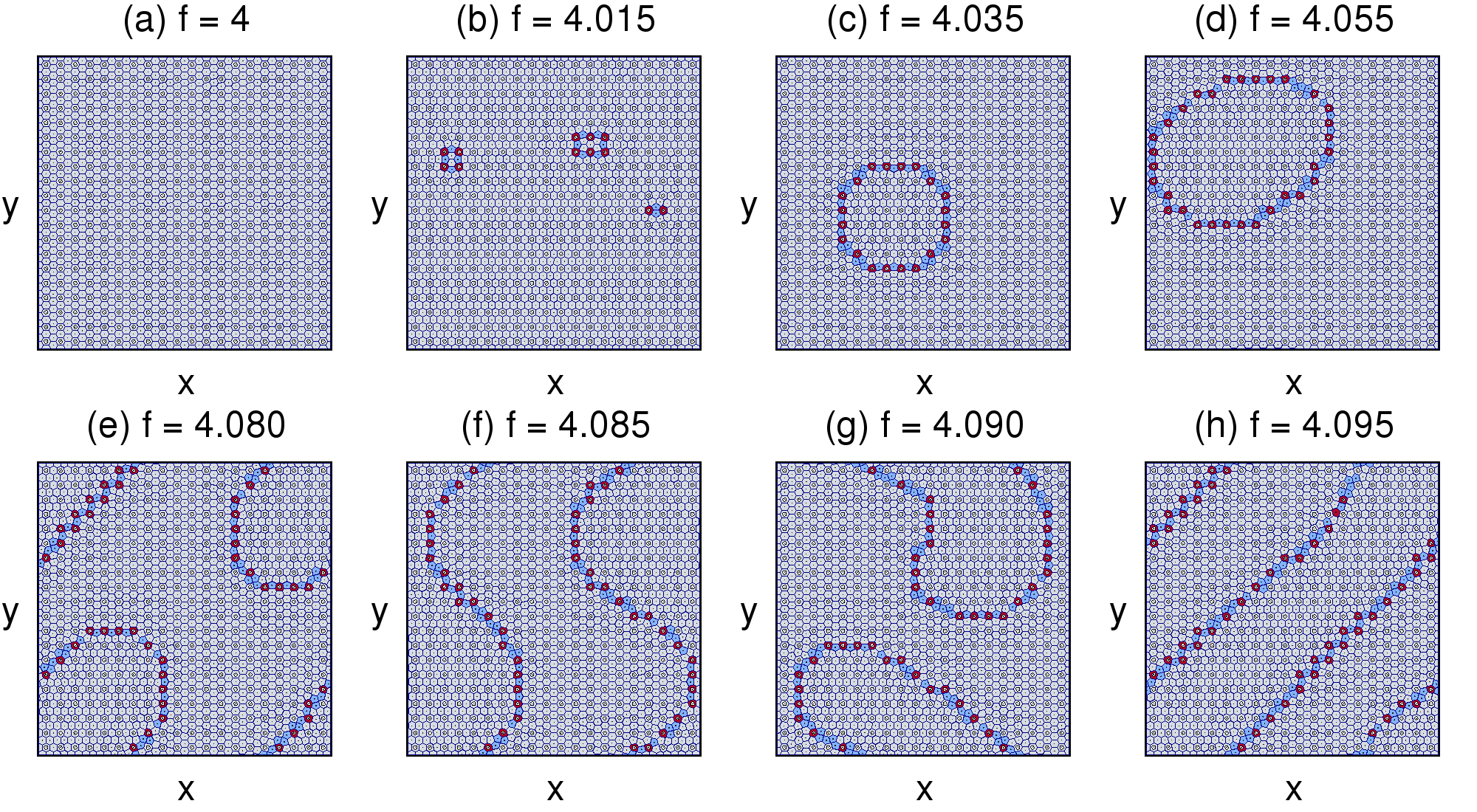
Fig. 1: The Voronoi diagrams of the colloidal particle configurations on a square pinning array. Filled dots: particle locations; open circles: pinning site locations. Polygon colors indicate the coordination number of the particle at the center of the polygon: 4 (dark blue), 5 (light blue), 6 (grey), or 7 (red). (a) At f=4, each pinning site captures one particle and a hexagonal lattice forms. (b) At f = 4.5, the particles form a superlattice structure with a periodicity of twice the pinning lattice unit cell. (c) At f = 5.0, a square lattice forms. 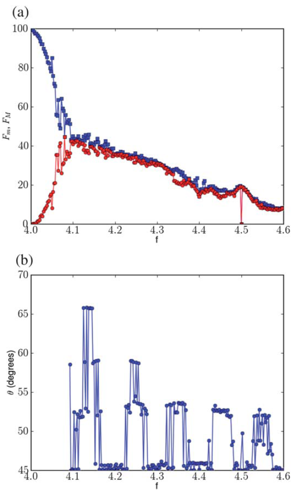(d) A stacked percentage chart of the fraction of particles with coordination number of 4 (dark blue), 5 (light blue), 6 (grey), and 7 (red) vs filling factor f showing how the system evolves from a hexagonal structure at f=4 to a square structure at f=5.

2 Simulation and System

We consider a two-dimensional system with periodic boundary conditions in x and y containing N_c colloidal particles with a density ρ = N_c/L², where L is the size of the sample in each direction. The particle-particle interaction is given by a Yukawa or screened Coulomb potential, and the colloids also interact with a square array of N_p pinning sites that are each of radius R_p. The filling fraction is f = N_c/N_p. The particle configurations are obtained by starting from a high temperature state and performing simulated annealing to reach a frozen state. The motion of particle i during the annealing arises from integrating the following overdamped equation of motion:

d R_i

= −

N_c
∑
i ≠ j

∇V(R_ij) + F^P_i + F^T_i

(1)

where η is the damping coefficient. The repulsive particle-particle Yukawa interaction potential is V(R_ij) = E₀exp(−κR_ij)/R_ij, where R_ij = |R_i − R_j|, R_i(j) is the position of particle i(j), E₀ = Z^*2/(4πϵϵ₀a₀), Z^* is the effective charge, ϵ is the solvent dielectric constant, and 1/κ is the screening length. The pinning interaction is modeled as arising from non-overlapping parabolic traps with F^P_i = ∑_k=1^N_pF_p(R_ik/R_p)Θ(R_p− R_ik)∧R_ik, where R_ik = |R_i − R_k| is the distance between particle i and the center of pinning site k located at R_k, ∧R_ik = (R_i − R_k)/R_ik, F_p is the maximum force of the pinning site, and Θ is the Heaviside step function. Our dimensionless simulation units are intended to represent micron-scale colloidal particles, and a system of the type we describe could readily be realized experimentally; for example, for a substrate lattice constant of 8 microns, the colloidal lattice constant at the f=5 matching field would be close to 3.75 microns, and in addition, substrates with a strength of up to 10 k_BT per trap have been created in experiment [15] The effects of thermal fluctuations are modeled by the Langevin term F^T in the form of randomly distributed thermal kicks with the properties 〈F^T(t)〉 = 0 and 〈F^T_i(t)F(t^′_j)〉 = 2ηk_Bδ_ijδ(t − t^′), where k_B is the Boltzmann constant. We have tested several annealing rates and work with a rate that is slow enough that no noticeable difference in the colloidal arrangement appears if an even slower rate is used. We have found that for fast annealing rates, the stripe patterns described below still form but contain grain boundaries instead of being fully oriented.

Fig. 2: The Voronoi diagrams with the same coloring convention as in Fig. 1 for fillings f = (a) 4.0, (b) 4.015, (c) 4.035, (d) 4.055, (e) 4.080, (f) 4.085, (g) 4.090, and (h) 4.095. In this disordered domain wall regime, the particles form grain boundaries of paired fivefold and sevenfold coordinated (5-7) defects separating different grain orientations.

3 Colloidal Particle Configurations

We concentrate on systems with N_p=400 and N_c=1600 to 2000, giving a filling fraction 4 ≤ f ≤ 5. At f = 4 each pinning site captures one particle while the remaining particles are located in the interstitial regions. The result is a hexagonal lattice structure in which all of the particles have exactly six neighbors. In Fig. 1(a) we plot the Voronoi diagram for the f = 4 state indicating the coordination number of each particle. Here, a hexagonal lattice forms and all particles are sixfold coordinated, while at f = 5.0, Fig. 1(c) shows that the particles form a square lattice with fourfold coordination. At f = 4.5 in Fig. 1(b), an exotic isotropic superlattice state appears consisting of alternating square arrangements of fivefold coordinated particles with a fourfold coordinated particle in the center and groups of six sixfold coordinated particles. The unit cell of the structure in Fig. 1(b) is twice the size of the pinning lattice unit cell.

We next address how the system evolves between the hexagonal and square orderings as f is varied from f=4 to f=5. In Fig. 1(d) we plot the fraction of particles with coordination number 4, 5, 6, and 7 for 4.0 ≤ f ≤ 5.0, showing that the system begins with hexagonal ordering and has a peak in the fraction of fivefold and sevenfold coordinated particles at f=4.5. For f > 4.65 we observe the rapid growth of the fraction of fourfold coordinated particles with increasing f until the system reaches a square lattice at f=5.0. We identify four regimes as a function of f: a disordered domain wall regime for 4.0 < f < 4.1, a stripe crystal regime for 4.1 ≤ f < 4.6, a disordered patchy regime for 4.6 ≤ f < 5.0, and the crystalline states at f = 4, 4.5, and 5.

In Fig. 2 we illustrate the domain wall regime for f = 4, 4.015, 4.035, 4.055, 4.080, 4.085, 4.090, and 4.095. In this regime, there are no individual defects; instead, pairs of fivefold and sevenfold coordinated (5-7) defects assemble into grain boundaries separating two different orientations of the hexagonal ordering. The grain boundaries grow in size until they span the entire system, as shown in Fig. 2(h) for f = 4.095. If we repeat the simulations using different initial randomizations of the temperature fluctuations, we obtain grain boundaries of the same general shape; however, the exact locations of the grain boundaries can differ.

Fig. 3: The Voronoi diagrams with the same coloring conventions as in Fig. 1 for fillings f = (a) 4.1, (b) 4.25, (c) 4.3, (d) 4.35, (e) 4.4, (f) 4.45, (g) 4.5, and (h) 4.55. Here the system forms stripe crystal states containing ordered lines of 5-7 defects, with the number of stripes increasing with increasing f. The orientation of the stripes with respect to the underlying pinning lattice varies with filling. At f=4.5 in panel (g), the system forms the isotropic superlattice structure.

In Fig. 3, we show particle configurations in the stripe regime for f = 4.1, 4.25, 4.3, 4.35, 4.4, 4.45, 4.5, and 4.55. Here the system forms stripe arrangements of 5-7 defects, where the number of stripes grows with increasing f, and with the isotropic superlattice structure appearing at f=4.5 in Fig. 3(g). As f changes, the orientation of the stripes with respect to the underlying pinning lattice can change, and the thickness of the stripes can vary. Some stripe states consist of one-dimensional lines, while in other stripe states, such as at f=4.1 in Fig. 3(a), there are zig-zag patterns. These patterns can even be combined, such as at f=4.4 in Fig. 3(e) where there are both zig-zag and one-dimensional lines of stripes. At f = 4.45 and f=4.55 in Fig. 3(f) and Fig. 3(h) there are two stripe structures that are interspersed. We find similar stripe patterns at these fillings in larger samples. Since the stripe directions are degenerate, it is possible that domains of different stripe orientation could form in the sample, as found for the ordering of repulsive particles such as superconducting vortices on periodic arrays for fillings below f=1 [20,21]. In our system, since most of the particles are not directly pinned by the pinning sites, they can move freely through the interstitial regions during the annealing process and can more readily fall into a global low energy state without different domains. In contrast, for f < 1 all the particles are directly pinned by the substrate and must hop from one site to another via thermal activation, producing much stronger kinetic constraints and making it more likely that domains of different orientation will be quenched into the sample. This result indicates that muffin tin potentials permit much larger ordered regions than can be obtained with egg-carton potentials.

Fig. 4: The Voronoi diagrams with the same coloring conventions as in Fig. 1 for fillings f = (a) 4.65, (b) 4.7, (c) 4.75, (d) 4.8, (e) 4.85, (f) 4.9, (g) 4.95, and (h) 5.0. Here the stripe structure is replaced by disordered patchy regions of square domains that grow in size with increasing f.

Figure 4 shows the evolution out of the stripe state into the disordered patch state at f = 4.65, 4.7, 4.75, 4.8, 4.85, 4.9, 4.95, and 5.0. The stripe state is still present at f = 4.6; however, at f = 4.65 in Fig. 4(a), patches of disorder begin to emerge, and at f = 4.70 in Fig. 4(b) some fourfold coordinated particles appear in patches that increase in size with increasing f before finally filling the entire system at f=5.0 in Fig. 4(h). The patches do not form regular stripelike patterns as seen for f < 4.6 but are more disordered, implying that the low energy state in this regime must be much more degenerate than in the stripe forming regime.

Fig. 5: (a) The fraction of particles in minority grains F_m (circles) and majority grains F_M (squares) vs f. For f < 4.1 the system is in the domain wall regime. When the two curves meet, the system enters the stripe regime. For f > 4.6, stripes can no longer be identified and the system enters the disordered patch regime. (b) Distribution of the stripe orientation angle θ with respect to the x axis vs f in the stripe regime. The stripes are predominantly aligned along θ = 45^°, 53^°, 59^°, and 66.8^°, corresponding to symmetry directions of the underlying square pinning array.

4 Analysis

In order to quantify where the different regimes occur, we have developed an algorithm to identify the grain boundaries and their orientation [27]. In the domain wall regime for 4.0 < f < 4.1, the sixfold coordinated particles in each domain can take one of two degenerate orientations. We define the majority grain direction to be the orientation of the largest domain in the sample, and the minority grain direction as the other degenerate orientation. We then measure the fraction of particles F_M that reside in domains with the majority orientation and the fraction of particles F_m in domains with the minority orientation. This definition is necessary since the majority grain direction can vary from one disorder realization to another. Figure 5(a) shows F_M and F_m versus f. Just above f = 4, there are small patches of minority grains, with most of the particles in one large majority grain. As f increases, F_M and F_m approach each other until meeting near f = 4.1 where the stripe regime begins. The stripe regime consists of crystalline states that have approximately equal quantities of grains of each orientation. The overall fraction of sixfold coordinated particles drops with increasing f as more stripe walls appear. Our grain boundary identification algorithm breaks down for f > 4.6 when the disordered patches appear, and also at f = 4.5 in the isotropic superlattice.

In Fig. 5(b) we plot the distribution of the angle θ between the stripe orientation and the x axis for the fillings 4.1 ≤ f < 4.6 where the stripes can be identified. There are four predominant angles, θ = 45^°, 53^°, 59^°, and 66.8^°. These angles can be written as θ = tan⁻¹(p/q) with integer p and q for p/q = 1, 4/3, 5/3, and 7/3, indicating that the stripes are aligning with symmetry directions of the underlying square pinning array. The other observed values of θ can also be matched to higher order rational ratios of p/q. The alignment of particle structures with the symmetry directions of an underlying pinning lattice has also been observed for colloidal particle ordering on quasicrystalline arrays [28] as well as for driven colloidal particles moving over periodic and quasicrystalline arrays [29,30,31]. Not all angles corresponding to possible rational values of p/q can be realized due to the fact that the domain walls are composed of 5-7 defects and therefore have a finite thickness.

Fig. 6: The energy distribution per particle P(E) vs f plotted using a color scheme where red indicates high values of P(E) and blue indicates low values of P(E). In both the grain boundary regime and the disordered patch regime, P(E) is broad, while in the crystalline stripe regime, P(E) is much narrower.

For each filling, we can determine the particle-particle interaction energy of each particle E_i=∑_{i ≠ j}^N_cV(R_ij) and then construct the distribution P(E) of the energy of all particles in the system. In Fig. 6 we plot the resulting P(E) versus f. For f < 4.1, P(E) has a maximum just above E = 6.2, corresponding to the per-particle energy associated with the hexagonal lattice at f = 4.0. As f increases, the peak in P(E) remains close to E=6.2 with some weight in P(E) shifting to higher energies due to the increasing fraction of grain boundaries in the sample. The highest energy particles are located along the grain boundaries. Once the system enters the stripe regime for 4.1 ≤ f < 4.6, P(E) becomes much narrower due to the strong crystalline ordering of the stripe phases, while the peak energy increases linearly with increasing E. In the disordered patch regime, P(E) broadens again, indicating that the particles form disordered states with many different particle-particle interaction energies. Just below and at f = 5.0, P(E) becomes very narrow again as the square lattice forms.

We can compare the stripe ordering to the pattern formation found on periodic egg-carton potentials such as vortex ordering in superconducting wire networks or colloidal particles on optical trap arrays for fillings f < 1.0 [20,21,22,23,24]. In these network systems, the f=1/3 filling for a square array produces a stripelike pattern of particles. This is contrast to our system, where the stripes are not individual particles but domains of non-sixfold coordinated particles. In the network systems, the ordering from 0 ≤ f ≤ 1/2 has a duality with 1/2 ≤ f ≤ 1, where the configurations for f=1/2 − x and f=1/2 + x are the same except that particle locations are replaced by void locations. In our system for 4.0 < f < 5.0, a similar duality does not occur. Additionally, at the higher fillings, the interstitial regions in the muffin tin potential allow particles to take positions that are inaccessible in egg-carton potentials.

Fig. 7: A stacked percentage chart of the fraction of particles with coordination number of 4 (dark blue), 5 (light blue), 6 (grey), and 7 (red) vs f over the range 1.0 ≤ f ≤ 9.0. Square lattices appear at f=1.0, 2.0, and 5.0, while hexagonal lattices form at f=4.0, 6.0, 8.0, and 9.0.

Fig. 8: The Voronoi diagrams with the same coloring conventions as in Fig. 1 for other fillings. (a) At f = 3.075, grain boundaries appear. (b) At f = 3.4, stripes form. (c) At f = 3.925, grain boundaries again form. (d) At f = 5.1 there is a disordered patch state. (e) At f = 5.35 a stripe state forms. (f) At f = 6.35 the system is disordered. (g) At f = 7.6, labyrinth type grain boundaries form. (h) At f=8.8, a particle stripe state appears.

5 Other fillings

We have also examined incommensurate fillings from f=1.0 to f=9.0. In Fig. 7 we show the fraction of particles with coordination number 4, 5, 6, and 7 versus f over this entire range. Square lattices occur at f=1.0, 2.0, and 5.0, with 100% of the particles fourfold coordinated at these fillings, while hexagonal lattices occur at f=4.0, 6.0, 8.0, and 9.0, with 100% of the particles sixfold coordinated at these fillings. At f=7.0 the system forms a patchy nonordered pattern, while at f=3.0 the interstitial colloidal particles form a dimer crystal arrangement with alternating dimer orientation. Figure 7 shows considerable fine structure at noninteger fillings, and certain types of superlattices form for some fillings as indicated by pronounced peaks and dips at f=3.5, 4.5, and 5.5. In general, we find that domain wall formation occurs at most incommensurate fillings; however, the morphology can exhibit differences depending on the closest integer filling. The best examples of stripe crystalline states appear between f=4 and f=5. In the range f=2 to f=3, the system forms only disordered patch states, and no grain boundaries could be identified, while between f=3 and f=4, the system exhibits grain boundary and stripe regimes but no disordered patchy regime. The ordering at f = 3 is not triangular or square but is instead a superlattice state. Figure 8(a) shows the grain boundary state at f = 3.075, Fig. 8(b) shows the stripe state at f = 3.4, and Fig. 8(c) shows that at f=3.925 a grain boundary state appears that is similar to that found at f = 4.05. For 5 < f < 6, the system exhibits disordered patch states of the type illustrated in Fig. 8(d) for f = 5.1, as well as stripe states where the stripes are aligned only along θ = 0^° or θ = 90^°, as shown in Fig. 8(e) for f = 5.35. For 6 < f < 7, the system does not form stripes but is instead disordered, as shown in Fig. 8(f) for f = 6.35. For 7 < f < 8, we mostly find labyrinth type grain boundary states such as that illustrated in Fig. 8(g) for n = 7.6, while for 8 < f < 9, the system mostly exhibits isolated defects in a triangular lattice, with some instances of stripelike domains as shown in Fig. 8(h) for f = 8.8.

In our study we have only considered square pinning arrays; however, the nature of the stripe and grain boundary states may change considerably for the case of hexagonal pinning arrays. Additionally, we have only explored the static states, but it is likely that the effective friction experienced by the particles under an applied drive can strongly affect the ordering of the particles, as has been recently demonstrated for domain wall formation in systems of colloidal particles interacting with periodic pinning arrays near the f=1 filling [32,33].

6 Conclusions

We have shown that a rich variety of distinct defect patterns occur for colloidal particles interacting with a square muffin tin potential array. The system forms a hexagonal lattice for four colloidal particles per pinning site and a square lattice for five colloidal particles per pinning site, and for intermediate fillings we identify a domain wall regime, a crystalline stripe regime, and a disordered patch regime. We show how these different regimes can be be distinguished with Voronoi diagrams, grain orientation measurements, and energy dispersion. These ordered defect patterns arise in the muffin tin potential due to the fact that a fraction of the colloidal particles are located in the interstitial regions between the pinning sites and have more mobility than particles on an egg-carton potential. We show that the pattern formation of the grain boundaries also occurs for a range of other fillings up to nine colloidal particles per trap, with the most prominent stripe crystalline states forming when there are between four and five colloidal particles per trap. Our results may provide a new method for tailoring defect structures in colloidal particle systems.

7 Acknowledgements

This work was carried out under the auspices of the NNSA of the U.S. DoE at LANL under Contract No. DE-AC52-06NA25396. D.M. and J.A. received support from the ASC Summer Workshop program at LANL.

References

[1]: A. Pertsinidis and X.S. Ling, Nature (London), 2001, 413, 147.
[2]: C. Reichhardt and C.J. Olson, Phys. Rev. Lett., 2002, 89, 078301.
[3]: A. Pertsinidis and X.S. Ling, Phys. Rev. Lett., 2008, 100, 028303.
[4]: S. Herrera-Velarde and H.H. von Grünberg, Soft Matter, 2009, 5, 391.
[5]: C. Bechinger, M. Brunner and P. Leiderer, Phys. Rev. Lett., 2001, 86, 930.
[6]: L. Radzihovsky, E. Frey, and D.R. Nelson, Phys. Rev. E, 2001, 63, 031503.
[7]: P. Tierno, Soft Matter, 2012, 8, 11443.
[8]: J. Baumgartl, M. Brunner, and C. Bechinger, Phys. Rev. Lett., 2004, 93, 168301.
[9]: C. Reichhardt and C.J. Olson Reichhardt, Phys. Rev. E, 2005, 72, 032401.
[10]: C. Reichhardt and C.J. Olson, Phys. Rev. Lett., 2002, 88, 248301.
[11]: M. Brunner and C. Bechinger, Phys. Rev. Lett., 2002, 88, 248302.
[12]: A. Sarlah, E. Frey, and T. Franosch, Phys. Rev. E, 2007, 75, 021402.
[13]: S. El Shawsish, J. Dobnikar, and E. Trizac, Soft Matter, 2008, 4, 1491.
[14]: C. Reichhardt and C.J. Olson Reichhardt, Phys. Rev. E, 2012, 85, 051401.
[15]: K. Mangold, P. Leiderer, and C. Bechinger, Phys. Rev. Lett., 2003, 90, 158302.
[16]: P.T. Korda, M.B. Taylor, and D.G. Grier, Phys. Rev. Lett., 2002, 89, 128301.
[17]: M.P. MacDonald, G.C. Spalding, and K. Dholakia, Nature (London), 2003, 426, 421.
[18]: K. Harada, O. Kamimura, H. Kasai, T. Matsuda, A. Tonomura, and V.V. Moshchalkov, Science, 1996, 274, 1167.
[19]: C. Reichhardt, C.J. Olson, and F. Nori, Phys. Rev. B, 1998, 57, 7937.
[20]: C. Reichhardt and N. Grønbech-Jensen, Phys. Rev. B, 2001, 63, 054510.
[21]: S. Bleil, H.H. von Grünberg, J. Dobnikar, R. Castañeda-Priego, and C. Bechinger, Europhys. Lett., 2006, 73, 450.
[22]: G.I. Watson, Physica A, 1997, 246, 253.
[23]: T.C. Halsey, Phys. Rev. B, 1985, 31, 5728.
[24]: S. Teitel and C. Jayaprakash, Phys. Rev. B, 1983, 27, 598.
[25]: P. Bak, Rep. Prog. Phys., 1982, 45, 587.
[26]: S.N. Coppersmith, D.S. Fisher, B.I. Haperin, P.A. Lee, and W.F. Brinkman, Phys. Rev. B, 1982, 25, 349.
[27]: J. Amelang and C.J. Olson Reichhardt, to be published.
[28]: J. Mikhael, G. Gera, T. Bohlein, and C. Bechinger, Soft Matter, 2011, 7, 1352.
[29]: C. Reichhardt and F. Nori, Phys. Rev. Lett., 1999, 82, 414.
[30]: C. Reichhardt and C.J. Olson Reichhardt, J. Phys.: Condens. Matter, 2012, 25, 225702.
[31]: T. Bohlein and C. Bechinger, Phys. Rev. Lett., 2012, 109, 058301.
[32]: T. Bohlein, J. Mikhael, and C. Bechinger, Nature Mater., 2012, 11, 126.
[33]: A. Vanossi, N. Manini, and E. Tosatti, arXiv:1208.4856.

File translated from T_EX by T_THgold, version 4.00.

Back to Home