Physical Review E 83, 061404 (2011)

Positive and Negative Drag, Dynamic Phases, and Commensurability in Coupled One-Dimensional Channels of Particles with Yukawa Interactions

C. Reichhardt¹, C. Bairnsfather^1,2, and C. J. Olson Reichhardt¹

¹Theoretical Division, Los Alamos National Laboratory, Los Alamos, New Mexico 87545, USA
² Department of Physics, Purdue University, West Lafayette, Indiana 47907, USA

(Received 8 December 2010; revised manuscript received 14 April 2011; published 13 June 2011)

We introduce a simple model consisting of two or three coupled one-dimensional channels of particles with Yukawa interactions. For the two channel system, when an external drive is applied only to the top or primary channel, we find a transition from locked flow where particles in both channels move together to decoupled flow where the particles in the secondary or undriven channel move at a slower velocity than the particles in the primary or driven channel. Pronounced commensurability effects in the decoupling transition occur when the ratio of the number of particles in the top and bottom channels is varied, and the coupling of the two channels is enhanced when this ratio is an integer or a rational fraction. Near the commensurate fillings, we find additional features in the velocity-force curves caused by the slipping of individual vacancies or incommensurations in the secondary channels. For three coupled channels, when only the top channel is driven we find a remarkably rich variety of distinct dynamic phases, including multiple decoupling and recoupling transitions. These transitions produce pronounced signatures in the velocity response of each channel. We also find regimes where a negative drag effect can be induced in one of the non-driven channels. The particles in this channel move in the opposite direction from the particles in the driven channel due to the mixing of the two different periodic frequencies produced by the discrete motion of the particles in the two other channels. In the two channel system, we also demonstrate a ratchet effect for the particles in the secondary channel when an asymmetric drive is applied to the primary channel. This ratchet effect is similar to that observed in superconducting vortex systems when there is a coupling between two different species of vortices.

I. INTRODUCTION
II. SIMULATION
III. TWO CHANNEL SYSTEMS
A. Coupling-Decoupling Transitions for Commensurate Channels
B. Dynamics and Commensurability
C. Finite Size and Temperature Effects
D. Ratchet Effect With ac Drives
IV. THREE CHANNEL SYSTEMS
A. Coupling-Decoupling Transitions for Partial Commensuration
B. Dynamics for Increased Incommensuration
C. Negative Drag
D. Unlocking of the Central Channel
E. Five Dynamical Phases
V. DISCUSSION AND SUMMARY
References

I. INTRODUCTION

There are many systems composed of repulsively interacting particles with one dimensional (1D) or quasi-1D motion, including colloids in narrow channels [1,2,3,4,5,6,7,8,9,10], Wigner crystal states in wires [11,12,13,14,15,16,17,18,19] and constrictions [20], dusty plasmas in grooves [21], macroscopic charged ball bearings in channels [22], and vortices in type-II superconductors confined within narrow strips or channels [23,24,25,26,27]. In many of these systems, interesting structural transitions from 1D lines of particles to zig-zag or buckled states can occur [17,4,19]. There can also be higher order transitions from 2 rows to 3 rows of particles or transitions to disordered states [23,24,5,27]. Under an external drive, this type of system also exhibits a variety of dynamical behavior such as ordered or disordered motion through constrictions [1,20,27] or dynamic commensurability effects [23,24].

Here we propose a simple system consisting of particles in two or three coupled 1D channels. The particles in each channel interact with the other particles in the same channel as well as with particles in adjacent channels via a Yukawa potential. An external drive applied to only one channel produces drag effects on the particles in the undriven channels, causing them to move. Our system is illustrated in Fig. 1. The two channel system is similar to the transformer geometry studied for vortices in two superconducting layers where an external drive is applied to one (primary) layer and the response of the nondriven (secondary) layer is measured [28,29,30]. If the vortices in the two layers are fully coupled, the response of the secondary layer is exactly the same as the response of the primary layer. If the vortices are only partially coupled, the response in the secondary layer is smaller than that of the primary layer. The transformer geometry has also been studied for vortex systems with multiple layers, such as vortices in the strongly layered high-temperature superconductors [31]. Drag effects have also been predicted for two coupled 1D wires containing classical 1D Wigner crystals when only one of the wires is driven [13]. In this case the interaction between particles in neighboring wires is repulsive, unlike the attractive interaction between vortices in neighboring layers. For the coupled 1D Wigner crystals there is also a transition from a completely locked state, where the response in both wires is identical, to a partially locked state, where the response of the secondary wire is reduced. Drag effects in coupled wire experiments have been interpreted as arising from the formation of Wigner crystal states [32].

Figure 1: Image of the sample geometry. The locations of the three channels are indicated by dotted lines. Black dots are particles within the channels. The arrow denotes the driving force which is applied only to particles within the top channel, termed the primary channel p. The bottom undriven channels are the secondary channels s₁ and s₂. The ratio of the number of particles in each channel is R_s1,p=N_s1/N_p and R_s2,p=N_s2/N_p, where N_s1 and N_s2 are the number of particles in the secondary channels and N_p=16 is the number of particles in the primary channel. The spacing between channels d is marked in panel (a). (a) Two channels with R_s1,p = 1.0 (b) Two channels with R_s1,p = 0.5. (c) Three channels with R_s1,p=1.0 and R_s2,p=1.0. (d) Three channels with R_s1,p=1.0 and R_s2,p = 1.5.

In this work we consider the effect of changing the ratio of the number of particles in each channel on the locking or coupling between the channels, with a particular focus on ratios that are integers or rational fractions. Commensuration effects [33] occur when the spacing between particles in one channel is a simple rational fraction of the spacing between particles in another channel, while incommensurations such as vacancies or interstitials appear when the two spacings are incommensurable. Commensuration effects have been studied extensively for systems in which a varied number of particles interacts with a rigid periodic substrate, such as atoms and molecules on surfaces [34], vortices in superconductors with periodic pinning arrays [35,36,37], and colloids interacting with 1D [38] or two-dimensional (2D) optical trap arrays [39], all of which can be viewed as physical realizations of the Frenkel-Kontrova model. These studies find that the coupling to the substrate or the effective pinning of the particles by the substrate is strongly enhanced when the ratio of the number of particles to the number of substrate minima is an integer or a rational fraction, as indicated by the appearance of peaks in the critical depinning force or enhanced ordering of the particles at the commensurate fillings. In our system, for the two channel geometry illustrated in Fig. 1 the particles in the secondary channel can be regarded as a distortable or moveable periodic pinning substrate for the particles in the primary channel, suggesting that enhanced drag or coupling could occur when the ratio of the number of particles in each channel is an integer or a rational fraction. The deformability of the substrate makes our proposed model distinct from Frenkel-Kontrova systems. Additionally, driven 1D and 2D commensurate-incommensurate systems often exhibit numerous dynamic behaviors within the incommensurate regimes, such as when localized vacancies or interstitials form soliton-like excitations which move more easily than the particles over the substrate [40,41]. This suggests that similar phases may be possible in the coupled channel drag system we propose here, and we show that such phases do appear. We also show that when we make the system more complex by adding a third channel, a remarkable variety of commensuration effects and dynamic regimes occur such as multiple decoupling, recoupling, and slip transitions, all of which produce pronounced changes in the velocity response. It is even possible to realize negative drag effects where the particles in one of the channels move in the direction opposite to that of the applied drive.

The coupled channels system we propose could be realized in colloidal systems. The number of colloids in the different channels can be controlled readily by optical manipulation and the colloids in one channel could be driven with an external field, optically, or using microfluidics. Another possible realization of this system is in nanowires where 1D Wigner crystallization of the electrons has occurred; in this case, by altering the electron density, the particle lattice spacing in one wire could be varied with respect to that in an adjacent wire. Realizing such a system could have important implications for the study of 1D Wigner crystals since the appearance of commensuration effects would be strong evidence that Wigner crystal states are forming. In superconducting systems, the density of magnetic vortices is fixed by the externally applied magnetic field, so it would be difficult to create 1D channels that contain different linear densities of vortices; however, in certain layered systems an additional transverse magnetic field can be applied to create a second Josephson vortex lattice which can interact with the pancake vortices in the planes [42,43,44]. It has already been shown that using this technique it is possible to drive only one of the vortex species and induce a drag on the other vortex species [43,44]. It should be possible to study fractional commensurate states in such a vortex system by examining how the drag effect changes when the ratio of the number of one type of vortices to the other is varied. A realization of three or more channels with varied numbers of particles in each channel should again be possible using colloidal systems or metallic wires. Further, a superconducting or nanowire system could be used in which each layer or channel has the same number of particles but differing amounts of quenched disorder. We note that there are previous studies of colloidal particles in 2D bilayers [45] where the particles in the layers are driven in opposite directions; however, these studies focused on an oscillatory order-disorder transition, not on the effects of commensuration on decoupling or the dynamic phases that we consider here for the case of 1D coupled channels.

The paper is organized as follows: In Section II, we describe our simulation method and sample geometry. We consider two channels of particles in Section III and illustrate a drive-induced decoupling transition for commensurate channels in Section III A. In Section III B we describe the two step decoupling transition that occurs for incommensurate channels which contain vacancy or interstitial sites that can act like a second species of particle. The effects of finite temperature and finite size appear in Section III C. Section III D shows that the nonlinear response of the system can be exploited to create a ratchet effect, where ac motion in the driven channel induces dc transport in the drag channel. In Section IV we turn to samples with three channels. We show in Section IV A that when the driven channel is commensurate with the neighboring drag channel, four different types of coupled and decoupled flow can occur as the occupancy of the second drag channel is varied, including regimes of intermittent coupling. In Section IV B, the driven channel is incommensurate with the neighboring drag channel and we find a complex series of coupling-decoupling transitions that produce a significant amount of structure in the velocity-force curves. In Section IV C, we consider in detail the negative drag that can occur at incommensurate fillings when the particles in one of the drag channels move in the direction opposite to the particles in the driven channel. It is also possible for the outer channels to remain coupled while the central channel is decoupled, as described in Section IV D. In Section IV E we summarize all five of the dynamical phases and the negative drag by showing that they can be achieved in a single system. The paper concludes in Section V with a discussion and summary.

II. SIMULATION

We model interacting Yukawa particles confined to move along 1D channels as illustrated in Fig. 1. Each particle interacts with other particles in the same channel and with particles in adjacent channels. The separation between channels is d=2 and, unless otherwise noted, there are N_p=16 particles in the driven or primary channel with a lattice spacing a, where L is the length of the channel. The particles in the primary channel p are coupled to an applied external driving force F_D. For a two channel system, the drag or secondary channel s₁ contains N_s1 particles, and the commensurability ratio is R_s1,p = N_s1/N_p. In a three channel system such as that shown in Fig. 1(c,d), the additional secondary channel s₂ is adjacent to s₁ but not to the primary channel p, and it contains N_s2 particles, giving a commensurability ratio of R_s2,p=N_s2/N_p.

The particle motions evolve under overdamped dynamics where the colloids obey the following equation of motion:

dR_i

= F^pp_i + F^D_p

(1)

Here η is the damping constant, R_i is the location of particle i, and the repulsive particle-particle interaction force is F^pp_i = ∑^N_v_{j ≠ i}−∇V(R_ij). The potential has a Yukawa or screened Coulomb form of

V(R_ij) =

E₀

R_ij

e^−κR_ij

(2)

with E₀ = Z^*2/4πϵϵ₀a₀, where ϵ is the solvent dielectric constant, Z^* is the effective charge, and 1/κ is the screening length. For colloidal systems, the length scale a₀ is on the order of a micron. We measure forces in units of F₀ = E₀/a₀ and time in units of τ = η/E₀. In a typical case, the distance between particles in channel p is a=2.25 while the distance between adjacent channels is d = 1.125a and the screening length is 1/κ = 2d, which is long enough to ensure strong coupling between the particles in all three channels. The driving force F^D_p=F_D∧x is applied only to all the particles in the primary channel. We increase F_D from zero in small increments of δF_D, holding the drive at constant values for a fixed time interval during which we measure the velocity of the particles in each channel. We have carefully checked that our waiting times are long enough to eliminate transient effects. We use δF_D = 0.001 and a wait time of 10⁵ simulation time steps. We impose periodic boundary conditions in the x-direction along the length of the channels. The velocity of the particles in the primary channel is given by V_p and the particle velocity in the secondary channels is given by V_s1 and V_s2. We normalize all the velocities by the number of particles in each channel, V_p=N_p⁻¹∑_i^N_pv_i, V_s1=N_s1⁻¹∑_i^N_s1v_i, and V_s2=N_s2⁻¹∑_i^N_s2v_i.

Figure 2: (a) The average velocity in the primary channel V_p and the secondary channel V_s1 vs F_D for a two channel system with R_s1,p = 1.0 and d/a = 0.67. The channels are locked for low F_D in the regime where V_p and V_s1 increase linearly. At F_D = 2.125, there is a transition to a partially decoupled state where the particles in the secondary channel begin to slip, producing a decreasing V_s1. (b) The decoupling force F_c force vs d/a for the system in (a) with R_s1,p=1, fixed d = 2.0, and a altered by changing the particle density. The decoupling transition drops to lower values of F_D as the particle density increases. (c) V_p (upper curve) and V_s1^′=N_p⁻¹∑_i^N_s1v_i (lower curve) vs F_D for the system in (a) but with R_s1,p = 0.92. Unlike the commensurate case in (a), the initial unlocking phase above F_D=1.04 is associated with the slipping of vacancies in s₁, while at F_D=2.25 there is a second unlocking transition above which all the particles in s₁ slip with respect to the particles in p. (d) V_p (upper curve) and V_s1^′ (lower curve) vs F_D for R_s1,p = 1.08, where the slipping at low drives is due to the presence of incommensurate particles.

III. TWO CHANNEL SYSTEMS

A. Coupling-Decoupling Transitions for Commensurate Channels

We first focus on the two channel system at commensurate filling with a particle ratio of R_s1,p = 1.0 and with d/a = 0.67. In Fig. 2(a) we plot V_p and V_s1 together versus F_D. Both V_p and V_s1 increase linearly with F_D for low F_D and have identical values, indicating that the motion in the two channels is locked. At F_D=2.125, we find a transition to a partially decoupled state where V_s1 monotonically decreases with increasing F_D while V_p continues to increase with F_D at a rate faster than the linear increase that occurred below the transition. The particles in s₁ are not completely decoupled from the primary channel since they still exhibit a nonzero velocity; since the particles in s₁ do not experience a driving force, they can move only due to interactions with the particles in p. Just above the decoupling transition, V_p increases with a square root form. The general shape of the velocity force curves in Fig. 2(a) is the same as that of the current-voltage curves obtained for superconducting transformer geometries [28,29,30,31], where the vortex velocities are proportional to the voltage and the applied current is proportional to the external force on the vortices in the primary channel. The current-voltage curves in the superconducting transformer system indicate that there is a drive-induced decoupling transition of the vortices in adjacent layers. In the vortex system, the vortex-vortex interaction between layers is attractive, so it is more intuitive why a finite vortex mobility persists in the secondary channel above decoupling. The results in Fig. 2(a) indicate that even when the particle-particle interactions are purely repulsive, a finite velocity in the secondary channel can be maintained at drives above the decoupling transition.

We measure the decoupling or unlocking force F_c as a function of d/a in a two channel system with R_s1,p = 1.0. The result is plotted in Fig. 2(b), where we fix d=2.0 and vary a by changing N_p and N_s1. Here F_c decreases with increasing particle density. A similar effect occurs in layered vortex systems, where for higher fields or higher vortex densities the coupling between the layers is gradually reduced [31]. For the Yukawa system this effect can be attributed to the reduced size of the periodic potential that the particles in s₁ experience from the particles in p. Once the primary channel is in motion, the particles in s₁ shift to positions that are slightly behind the driven particles. As the drive increases, the size of this shift increases until the particles in p slip more than 0.5a ahead of the particles in s₁, producing the partial decoupling. When the particle density increases, the amount of shift required to pass the position 0.5a decreases since a decreases with increasing particle density in both channels.

B. Dynamics and Commensurability

In Fig. 2(c) we plot V_p and V_s1^′ for a two channel system with R_s1,p = 0.92, where the number of particles in s₁ is smaller than the number of particles in p. Here V_s1^′=N_p⁻¹∑_i^N_s1v_i is the velocity of the particles in s₁ normalized by N_p, the number of particles in p. For low F_D the channels are locked and all of the particles in the system move at the same velocity. The slope of V_s1^′ versus F_D is slightly smaller than the slope of V_p versus F_D in Fig. 2(c) due to the fact that N_s1 < N_p. At F_D = 1.04 we observe a transition to a partially coupled state; however, this transition occurs at a drive well below the decoupling transition F_c=2.125 shown for the commensurate system in Fig. 2(a). Additionally, just above F_D=1.04, Fig. 2(c) indicates that the velocity-force curve does not have the characteristic square root shape found close to F_c in Fig. 2(a). For F_D > 1.04, V_s1^′ continues to increase with increasing F_D but with a smaller slope than in the locked regime. A second decoupling transition appears at F_D = 2.25. For F_D > 2.25, V_s1^′ decreases with increasing F_D and there is also a corresponding increase in the slope of V_p. The second decoupling transition occurs at a drive close to the value F_c=2.125 where decoupling of the commensurate system occurs, as shown in Fig. 2(a). This indicates that the second decoupling transition for the incommensurate system is the same as the sole decoupling transition found in the commensurate system, where all the particles in s₁ begin to slip with respect to the particles in p. The two step decoupling transition for the incommensurate system appears due to the presence of vacancies in s₁. At commensuration, all of the particles in s₁ are located within potential minima created by the spacing of the particles in p. Below commensuration, a fraction of the sites in this periodic potential are empty, producing effective vacancies in s₁. In the locked phase at F_D < 1.04, all the particles in s₁ move at the same velocity as the particles in p. At the first decoupling transition, the vacancies in s₁ begin to slip with respect to the particles in p. This can be viewed as a depinning transition. Every time a vacancy slips, only one of the particles in s₁ slips with respect to p while the remaining particles in s₁ stay locked with p. As a result, most of the particles in s₁ continue to increase in velocity with increasing F_D. For drives above the second decoupling transition, all of the particles in s₁ slip with respect to p and the slipping is no longer dominated by the motion of vacancies.

In Fig. 2(d) we plot V_p and V_s1^′ versus F_D for the same system in Fig. 2(c) but with R_s1,p = 1.08, where N_s1 > N_p so that a few incommensurate particles appear in s₁. The overall shape of the velocity-force curve in this case is very similar to that for R_s1,p = 0.92 shown in Fig. 2(c), with a first decoupling occurring at a lower drive of F_D = 0.6 than that for R_s1,p = 0.92, and a second decoupling transition occurring close to F_D = 2.0. Here the incommensurations in s₁ form doubly occupied sites in the periodic potential created by the particles in p. At R_s1,p=0.92 when there are vacancies in s₁, slipping of a particle adjacent to a vacancy occurs because the particle is able to move closer to the barrier separating two minima in the periodic potential. This is because the force the particle experiences on one side from a neighboring particle in s₁ is not compensated due to the missing particle at the vacancy site. As a result, there is an extra force of the order of F^pp(a) on the slipping particle, where a is the lattice constant of the particles in p. For the doubly occupied sites at R_s1,p=1.08, a similar situation occurs; however, the slipping particle in s₁ is located at a doubly occupied site and feels an uncompensated force from the other particle located within the same site. The extra force in this case is F_pp(a^′), where a^′ < a in order for the site to be doubly occupied. Thus, F_pp(a^′) < F_pp(a), so the initial decoupling transition occurs at a lower value of F_D for samples with R_s1,p > 1 that have incommensurations than for samples with R_s1,p < 1 that contain vacancies.

The appearance of multiple decoupling transitions just below and above commensuration and only one transition at commensuration is similar to the single and multiple depinning transitions observed in vortex systems [40] and colloidal systems [46] with periodic potentials at and near commensuration. In these 2D systems, at the matching filling of 1 particle per substrate minimum there is a single transition from a pinned state to a flowing state, while at fillings slightly away from commensuration, well-defined vacancies or interstitial particles appear which are highly mobile and depin at a lower external drive than the commensurate particles. The 2D systems are generally more complicated and allow for more than two depinning transitions near but not at commensuration [40]; however, as in our 1D case, it is the presence of two types of particles, the commensurate particles and the interstitial or vacancy sites, that produce the multiple depinning transitions. There are some important differences between our two channel system and the 2D vortex and colloidal systems. Our system contains no fixed periodic substrate so there is no pinned phase; however, there is a moving fully coupled state which is analogous to the pinned state. The regime in which the vacancies or incommensurations slip is then analogous to the depinning transitions of interstitials or vacancies, and the high driving phases at which all the particles are slipping corresponds to the completely depinned regime in the 2D systems.

Figure 3: (a) The velocity v of a single particle in s₁ vs time for the commensurate system in Fig. 2(a) at R_s1,p = 1.0 and F_D = 2.25. (b) The Fourier transform S(f) of the signal in panel (a) shows a well-defined characteristic frequency. (c) v(t) for a system with R_s1,p = 1.08 at F_D = 0.65. (d) The corresponding S(f) shows that there are two frequencies present. (e) v(t) for a system with R_s1,p = 0.92 at F_D=1.1. (f) The corresponding S(f) shows the presence of two frequencies.

In order to show more clearly that the particles in s₁ are experiencing a periodic potential produced by the particles in p and that there are two effective types of particles in s₁ away from commensuration, in Fig. 3(a) we plot the time trace of the velocity v(t) of a single particle in s₁ for the system in Fig. 2(a) at R_s1,p = 1.0 in the locked phase at F_D = 2.25. The value of v(t) is nearly constant except during the periodic slip events, during which v drops briefly below zero indicating that the particle temporarily moves backwards. In Fig. 3(b) we show the Fourier transform S(f) of v(t) highlighting the presence of a single characteristic frequency determined by the slipping events. In the locked phase, there is no high-frequency oscillation of the velocity of any of the particles. In Fig. 3(c) we plot v(t) for the system with R_s1,p = 1.08 from Fig. 2(d) at F_D = 0.65 where the channels are not completely locked but where V_s1^′ is still increasing with increasing F_D, and in Fig. 3(d) we show S(f) for the same data. There are now two frequencies present. The lower frequency is produced by the same slipping events that occurred for the commensurate system in Fig. 3(a,b), while the higher frequency originates from the motion of the incommensuration through s₁. In Fig. 3(e,f) we plot v(t) and S(f) for a sample with R_s1,p = 0.92 at F_D = 1.1. Again, there are two characteristic frequencies. The lower frequency is associated with the same slipping events shown previously, while the higher frequency is produced by the motion of a vacancy through s₁, rather than by the motion of an incommensuration.

Figure 4: V_p (upper curve) and V_s1 (lower curve) vs F_D for the two channel system from Fig. 2(a). (a) At R_s1,p = 0.5, there is a single transition from the completely coupled state to the partially decoupled state. (b) At R_s1,p = 0.58 there are two transitions. The first decoupling transition occurs when the incommensurations begin to slip while the other particles in s₁ remain locked with p. (c) At R_s1,p = 2.0 there is a single transition out of the locked phase. (d) At R_s1,p=1.92 (upper V_s1 curve) and R_s1,p = 2.08 (lower V_s1 curve) there is no locked phase, but there is still a local maximum in V_s1 which is higher for R_s1,p = 1.92.

The two stage decoupling process is most pronounced for fillings close to R_s1,p = 1.0, but the same effects appear near certain fractional ratios. For example, in Fig. 4(a) we plot V_p and V_s1 versus F_D for a sample with R_s1,p = 0.5 which has a single sharp decoupling transition at F_D = 1.9. Just above this filling at R_s1,p=0.58, shown in Fig. 4(b), there is an initial decoupling transition of the incommensurations near F_D = 1.5 into a state where V_s1 still increases with increasing F_D but with a greatly reduced slope. A second decoupling transition appears at F_D = 1.8, and above this drive V_s1 decreases with increasing F_D. In this case, incommensurations appear with respect to the particle configuration that occurs at R_s1,p=0.5. There is a single frequency associated with the motion of the particles in s₁ for R_s1,p=0.5, while for the incommensurate case of R_s1,p=0.58, two frequencies are present. This trend persists for higher values of R_s1,p as shown in Fig. 4(c) at R_s1,p = 2.0. Here there is a single sharp decoupling transition, while just below and just above this filling at R_s1,p = 1.92 and R_s1,p=2.08, Fig. 4(d) shows that the locking phase is absent but that a strong local maximum in V_s1 appears at F_D = 0.19 for R_s1,p = 1.92 and at F_D = 0.125 for R_s1,p = 2.08.

Figure 5: The force F_c at the transition from the locked to unlocked phase vs R_s1,p in two channel samples with different values of a. (a) At d/a=0.44, commensuration peaks occur at R_s1,p = 1.0, 2.0, and 3.0. Fractional peaks and anomalies appear at R_s1,p = 0.5, 1.5, and 2.5. (b) At d/a=0.67, there are commensuration peaks at R_s1,p = 0.5, 1.0, 1.5, and 2.0. (c) At d/a = 1.0, the strongest commensuration peaks appear at R_s1,p=1 and 0.5.

By performing a series of simulations for varied R_s1,p, we determine the location F_c of the transition from complete locking to a decoupled state and map out where the commensuration effects occur. In Fig. 5(a), we plot the decoupling force F_c versus R_s1,p for a two channel sample with d/a = 0.44, which falls in the strong coupling regime in Fig. 2(b). There are peaks in F_c at R_s1,p = 1.0, 2.0, and 3.0, along with submatching peaks at R_s1,p = 1/3, 1/2, and 2/3. Additionally, weaker anomalies appear at R_s1,p=1.5 and 2.5. In Fig. 5(b) we show F_c versus R_s1,p for a sample with d/a = 0.67. The value of F_c at the commensurate filling of R_s1,p=1.0 is lower for the d/a=0.67 sample than for the d/a=0.44 sample. Figure 5(b) also has clear peaks in F_c at R_s1,p = 2.0, 1.5, and 0.5, while above R_s1,p=2.0 within our resolution there are no peaks or regions where the system is locked. In the regions with F_c=0 where the locked phase is absent, the second decoupling transition still appears at higher drives and can be detected as the point at which V_s1 changes from increasing to decreasing with increasing F_D. For higher particle densities and fixed d, the commensurability effects still persist as shown in Fig. 5(c) for d/a = 1.0. Here, peaks in F_c occur at R_s1,p = 0.5, 1.0, and 2.0.

The appearance of the commensuration effects at integer and fractional fillings suggests that this system exhibits the same behavior found for the depinning of repulsively interacting particles on a 1D fixed periodic potential; however, there are several differences between the two systems. For particles on a fixed periodic potential, the depinning force F_c at fields where the particle-particle interactions cancel due to symmetry equals the maximum value of the pinning force F_p so that F_c = F_p at fillings 1/12, 1/8, 1/6, 1/4, 1/2, and 1.0. For the drag system shown in Fig. 5, this does not occur and there is even a trend for F_c to increase at the lowest fillings. This is because the substrate potential created by the particles in p is not fixed but can distort since the particles in either channel can shift. At R_s1,p = 1.0, the periodic potential is fairly rigid due to the matching of the particle positions in p and s1, and any distortion of the particles in p is energetically unfavorable. In contrast, at very low fillings such as R_s1,p=0.125, the particles in p distort near the locations of the particles in s₁ in order to create a localized lowering of the density in p above each particle in s₁. As a result, the particles in s₁ no longer experience the same periodic potential from p that was present for the commensurate case of R_s1,p=1.0. Even at R_s1,p = 0.5, the particles in p can distort, reducing the strength of the coupling to the particles in s₁.

Figure 6: V_s1 vs F_D for the system in Fig. 5(b) with d/a=0.67. (a) R_s1,p = 0.562, 0.625, 0.6875, and 0.75, from top to bottom. Inset: Detail of the R_s1,p=0.6875 curve from the main panel. (b) R_s1,p = 0.8125, 0.875, 0.9375, and 1.0, from bottom to top. (c) R_s1,p = 1.0625, 1.125, 1.1875, and 1.25, from top to bottom.

In order to better understand the changes in dynamics at the different fillings, in Fig. 6 we plot V_s1 as a function of F_D for varied R_s1,p in a system with d/a=0.67. At R_s1,p=0.5, a single decoupling transition occurs and V_s1 is a monotonically decreasing function. For R_s1,p = 0.562 and 0.625, shown in Fig. 6(a), there is a clear double peak structure in V_s1 with one peak falling at the depinning of the incommensurations and the second peak appearing at the unlocking transition. At R_s1,p = 0.6875 in Fig. 6(a), there is now a three peak structure in V_s1. The first peak, shown in the inset of Fig. 6(a), falls at the transition out of the completely locked phase at F_D = 0.11. The second and largest peak is at F_D = 0.3, while a third broad peak also appears that is centered at F_D = 1.45. The broad peak is the remnant of the second peak in V_s1 found for R_s1,p = 0.562 and 0.625; with increasing R_s1,p, this peak broadens and the center shifts to higher values of F_D. For 0.11 < F_D < 0.3, the particles in s₁ are almost completely locked but there is a single incommensuration which has begun to slip. For R_s1,p = 0.75, the initial peak is lost and the decoupling transition peak now falls at F_D=0.11. There is also a very broad maximum centered at F_D = 4.0. Another interesting feature is that at higher F_D such as at F_D = 6.0, V_s1 for R_s1,p = 0.75 is higher than V_s1 at the lower values of R_s1,p, even though at low F_D R_s1,p showed the lowest value of V_s1. This suggests that at high values of F_D, additional drag is produced by the interaction between the incommensurations in s₁ and the particles in p.

In Fig. 6(b) we plot V_s1 versus F_D for R_s1,p = 0.8125, 0.875, 0.9375, and 1.0. The maximum value of V_s1 increases as R_s1,p increases toward R_s1,p = 1.0 and the broad maximum in V_s1 sharpens and shifts toward lower F_D. Here, R_s1,p=1.0 has the lowest value and R_s1,p=0.8125 has the highest value of V_s1 at F_D = 6.0. In Fig. 6(c) we show V_s1 versus F_D for R_s1,p = 1.0625, 1.125, 1.1875, and 1.25. For these values of R_s1,p there is no completely locked phase; however, there is still a peak feature in V_s1 for R_s1,p = 1.0625 and 1.125 which broadens and shifts to higher F_D for increasing R_s1,p. At R_s1,p = 2.0 a locked phase reappears and the shape of V_s1 versus F_D is very similar to the curve shown for R_s1,p = 1.0.

Figure 7: V_s1 vs R_s1,p at F_D = 6.0 for the two channel system with d/a=0.67. Here the peaks appear not at the commensurate fields of R_s1,p = 1.0 and R_s1,p = 0.5 but at R_s1,p = 0.8 and R_s1,p=0.45. (b) V_s1^max vs R_s1,p obtained for each filling at the F_D where V_s1 reaches its maximum value. The peak centered at R_s1,p = 1.0 is much broader than the peak in F_c at R_s1,p=1.0 shown in Fig. 5(b).

In Fig. 7(a) we plot V_s1 versus R_s1,p at a fixed drive of F_D = 6.0 for the system in Fig. 6 with d/a=0.67. Larger values of V_s1 indicate that the particles in s₁ are exerting a larger drag on the particles in p. Here, peaks fall at R_s1,p = 0.45 and R_s1,p = 0.8, rather than at the values R_s1,p=0.5 and R_s1,p=1.0 where peaks appeared in F_c in Fig. 5(b). This shows that at high drives, the drag by the s₁ particles is the most effective away from the commensurate fillings. The curves shown in Fig. 6 indicate that if V_s1 were measured at a lower value of F_D, the peaks in Fig. 7(a) would shift closer to R_s1,p = 0.5 and 1.0.

In vortex systems with 2D periodic pinning arrays, experiments have shown that the pinning is enhanced at the matching fields as indicated by dips in the resistivity for low applied drives. For vortices that are strongly driven, however, the resistivity dips were found to shift away from the integer matching fields [47]. The interpretation was that at the matching fields in the highly driven system, the vortices form a very ordered moving commensurate state, while at the incommensurate fields the moving state is not as well ordered and thus the effectiveness of the pinning increases away from commensuration at high drives. Although the disorder in the incommensurate state causes the system to begin slipping at a lower drive for incommensurate fields, at high drives the disordered state experiences more fluctuations than the ordered state which induce some additional drag.

In Fig. 7(b) we plot V_s1^max versus R_s1,p. Here the measurement of V_s1^max is performed not at a fixed F_D but at the F_D where V_s1 reaches its maximum for each value of R_s1,p. In this case, a strong peak in V_s1^max appears at R_s1,p = 1.0. This peak is wider than the peak in F_c at R_s1,p=1.0 in Fig. 5(b) due to the fact that the maximum value of V_s1 increases as R_s1,p = 1.0 is approached, as shown in Fig. 6(b,c).

Figure 8: (a) F_c vs R_s1,p for the system with d/a = 0.67 from Fig. 5(b) of length L (diamonds), 2L (squares, curve shifted up by 0.4), and 4L (circles, curve shifted up by 0.8). For the larger systems, higher order fractional peaks appear at R_s1,p = 1/4, 1/3, 1/2, 2/3, 3/4, and 3/2. (b) The same data plotted without vertical shifts, for system sizes of L (diamonds), 2L (squares), and 4L (plus signs). Connecting lines are drawn only for the 4L system. The curves overlap exactly and the values of F_c are unaffected by system size. (c,d) V_s1 vs F_D for the 4L system from (a) at (c) R_s1,p = 1.0 and (d) R_s1,p = 0.896 for temperatures of T = 0.0, 0.22, 0.88, 2.0, and 4.5, from top to bottom. The decoupling transition drops to lower F_D with increasing T, while the drag effects persist up to high temperatures.

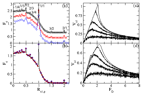
C. Finite Size and Temperature Effects

To determine whether further higher order submatching effects in R_s1,p can be resolved for larger systems and whether the values of F_D at which the unlocking transitions occur change with system size, we consider the system at d/a = 0.67 from Fig. 5(b) and analyze F_c for samples of size 2L and 4L. Here we hold a fixed by increasing N_p to 32 and 64, respectively. In Fig. 8(a) we plot F_c versus R_s1,p for samples of size L, 2L, and 4L, with the curves shifted vertically for clarity. In the larger samples, there are clearly fractional peaks falling at R_s1,p = 1/4, 1/3, 1/2, 2/3, 3/4, and 3/2. The 4L sample even shows some evidence of a peak at R_s1,p = 1/8. We expect that for even larger systems, even more fractional peaks will appear but that the higher order peaks will be increasingly weak in size, similar to the behavior of fractional peaks observed in other systems such as vortices on periodic substrates [35,36]. In Fig. 8(b) we plot the same data without vertical shifts to show that the depinning thresholds for the three systems overlap exactly; only the resolution is changed by the system size. We find no changes in the velocity-force curves as the size of the sample is increased, indicating that the system sizes we are studying capture the essential behavior. We also find a similar lack of dependence on sample size for the three layer systems that are described in Section IV. We note that for commensurate-incommensurate systems such as the Frenkel-Kontrova model [33], submatching effects theoretically occur for all rational values of m/n, where m is the number of particles and n is the number of substrate minima. In the Frenkel-Kontrova model, true incommensurate behavior occurs only for systems of infinite size at irrational filling ratios. In our system the higher order submatching effects are destroyed due to the fact that we do not have a fixed substrate; instead, the effective substrate experienced by the particles in one channel due to the presence of particles in the neighboring channel is able to distort. As a result, our system does not map directly onto commensurate-incommensurate systems such as the Frenkel-Kontrova model, although it displays several similarities with such models as we have shown.

In an experimental realization of the system we propose, such as with colloids confined to channels, thermal effects will be present. To test the stability of the different regimes we observe against thermal perturbations, we have performed simulations with the 4L system with d/a=0.67 at R_s1,p = 1.0 and R_s1,p = 0.896 at finite temperature. We use the same procedure employed in previous works to model the thermal fluctuations [48]. We add a Langevin noise term F^T_i to the equation of motion with the properties 〈F^T_i(t)〉 = 0 and 〈F^T_i(t)F^T_j(t′)〉 = 2ηk_B T δ_ijδ(t−t′). Fig. 8(c) illustrates V_s1 versus F_D at R_s1,p = 1.0 and Fig. 8(d) shows V_s1 versus F_D at R_s1,p = 0.896 for T = 0.0, 0.22, 0.88, 2.0, and 4.5. As the temperature increases, the value of F_c decreases until for T > 2.0 the locked phase has almost completely vanished; however, drag effects on the secondary channel continue to persist up to much higher temperatures. For R_s1,p = 0.896, the locking phase is lost at lower T than for R_s1,p=1.0 due to the fact that the effective incommensurations are more mobile and hence require a smaller level of thermal fluctuations to escape from the potential minima. These results show that the drag and locking features described for the zero temperature system should persist under finite temperature provided that the thermal fluctuations are not excessively strong.

Possible experimental realizations of the two channel system include modified versions of the colloidal experiments which have already been performed on coupled one-dimensional channels [9]. Colloidal systems are subject to thermal fluctuations and hydrodynamic interactions which can arise in the surrounding fluid. We showed above that the dynamic phases are robust against moderate thermal fluctuations. There is ongoing discussion regarding how the inclusion of hydrodynamic effects would impact the dynamics of driven colloidal systems. Recent two-dimensional simulations of an electrophoretically driven charged colloidal system similar to the one we consider showed that when the charge on the colloids are sufficiently strong, the dynamical behavior of the system is not altered by the addition of hydrodynamic interactions [49]. Due to the good agreement that has been found between numerous simulations of driven colloid systems in which hydrodynamic effects are neglected and the actual behavior of driven colloids in experiment, we expect that at least some of the features that we describe should be observable in a colloidal realization of this system. Another possible realization would be to generalize the recent experiments performed with dusty plasmas interacting with a one-dimensional groove to create what are termed Yukawa chains [21]. If more than one groove were created in the substrate, it should be possible to couple two or more of the Yukawa chains, to use a laser to drive one of the chains, and then to analyze the response of the secondary chain. In this case inertial effects could modify the behavior since dusty plasma systems are generally not in the overdamped limit.

D. Ratchet Effect With ac Drives

We next show that when the particles in p are driven with an ac drive, it is possible to generate a net dc motion of the particles in s₁ or a ratchet effect. Ratchet effects produced by applied ac drives have been studied extensively in systems of particles interacting with asymmetric substrates [50]; however, it is also possible to create a ratchet effect in the absence of an asymmetric substrate when the ac drive has certain asymmetries and when the response of the system is nonlinear [42,51,43,44]. This type of ratchet has been realized in systems with two interacting species of superconducting vortices such as when Josephson vortices couple to pancake vortices [42,43,44], as well as in interacting binary colloidal systems where only one colloid species couples to an external driving field and produces a rectification of the other colloid species [51].

Figure 9: Inset: Schematic of the ac force applied to p. Each period τ is divided into two parts. A force F_A is applied in the positive direction for a duration τ_A, then a force F_B is applied in the negative direction for a duration τ_B, with the condition that F_B/F_A = τ_A/τ_B = 4.0. Main panel: Induced dc velocity V_s1 averaged over multiple ac drive periods vs F_A for a two channel system with d/a = 0.67 under the applied ac drive shown schematically in the inset. Upper curve: R_s1,p=1.0; middle curve: R_s1,p=0.75; lower curve: R_s1,p=1.25. Here the ratchet effect reaches its maximum value for R_s1,p = 1.0. Within this range of F_A, V_p = 0 when averaged over an ac drive period.

Here we consider an ac square drive applied only to p. The period τ of the square drive is divided unevenly into two parts as illustrated in the inset of Fig. 9. In part A, we apply a force F_D=F_A∧x in the positive direction for a duration τ_A, while in part B we apply a force F_D=−F_B∧x in the negative direction for a duration τ_B=τ−τ_A. In selecting F_A and F_B, we impose the condition F_Aτ_A − F_Bτ_B=0 so that there is no net dc drive. If the response of the system is perfectly linear, this drive will not generate a net dc motion of the particles in either channel. On the other hand, if the coupling between s₁ and p is nonlinear, it is possible to induce a dc motion of the particles in s₁ by applying this ac drive to the particles in p. If both F_A and F_B are below the first decoupling transition F_c, the motion of the particles in both channels is completely locked, the response is perfectly linear, and there is no ratchet effect. If F_A < F_c and F_B > F_c, a net dc drift of the particles in s₁ will occur since the particles in s₁ remain completely locked with the particles in p during part A of the drive cycle, but during part B of the cycle the particles in s₁ are partially decoupled and do not move all the way back to their starting position by the end of the cycle.

In Fig. 9 we illustrate the ratchet effect which produces a finite positive value of V_s1 under the ac drive described above. We fix F_B/F_A=4.0 and d/a=0.67, and plot the time-averaged V_s1 versus F_A for R_s1,p = 0.75, 1.0, and 1.25. For low F_A, V_s1 starts small but rapidly grows with increasing F_A, reaching a sharp peak for R_s1,p = 0.75 and R_s1,p=1.0. As F_A increases above this peak, V_s1 gradually decreases with increasing F_A since the drag effect becomes smaller for higher drives as shown in Fig. 2(a). For R_s1,p = 1.25, the ratchet effect is strongly reduced but still persists, indicating that the ratchet effect should be a robust feature for all fillings. In all cases there is no induced dc flow of the particles in p. Our system can be regarded as containing two species of particles: the directly driven particles in p, and the undriven particles in s₁ that experience a drag from the particles in p. It would be very interesting to look for a similar ratchet effect in coupled quantum wires in the regime where Wigner crystallization may be occurring. This could be achieved by applying an ac drive of the type illustrated in the inset of Fig. 9 to one wire and determining whether a dc response is induced in the second wire.

Figure 10: The velocities V_p, V_s1, and V_s2 vs F_D for a three channel system with d/a=0.67, R_s1,p = 1.0, and varied R_s2,s1. (a) At R_s2,s1 = 1.0 there is a single transition from the locked region I to region II where the particles in s₁ and s₂ remain locked with each other but partially decouple from the particles in p. (b) At R_s2,s1 = 1.16 there is a transition from the locked region I to region III where the particles in s1 and p lock together but the particles in s₂ partially decouple. In region IV all three channels are unlocked, while at high F_D the system enters region II when the particles in s₁ lock with the particles in s₂ but are partially decoupled from the particles in p. (c) At R_s2,s1 = 1.5 the transition between regions IV and II occurs at a much higher value of F_D.

IV. THREE CHANNEL SYSTEMS

A. Coupling-Decoupling Transitions for Partial Commensuration

We next consider a system with three channels of particles where only the top channel is subjected to a driving force. We measure the velocities in each channel, denoted by V_p, V_s1, and V_s2, for particle ratios of R_s1,p = N_s1/N_p, R_s2,p = N_s2/N_p, and R_s2,s1 = N_s2/N_s1. For the commensurate case when all channels contain the same number of particles, R_s1,p = R_s2,p = R_s2,s1 = 1.0, the behavior is the same as in the two channel case at commensuration. There is a single decoupling transition from region I, the completely locked phase, to region II, where the particles in s₁ and s₂ remain locked with each other but are partially decoupled from the particles in p. This is illustrated in the plot of V_p, V_s1, and V_s2 versus F_D in Fig. 10(a) for a sample with d/a = 0.67, R_s1,p=1.0, and R_s2,s1=1.0. The decoupling between the primary and the secondary channels occurs at F_D = 1.75. The value of F_D at decoupling is lower than for a sample containing only two channels since the primary channel must now drag twice as many secondary particles.

In Fig. 10(b) we plot the channel velocities versus F_D for a sample with R_s1,p=1.0 but with more particles in s₂, R_s2,s1 = 1.16. For F_D < 0.37 the system is in the completely locked region I, while for 0.37 ≤ F_D < 1.625 the particles in p and s₁ remain locked but the particles in s₂ partially decouple. We term this range of F_D region III, and in this region V_s2 still increases with increasing F_D. For 1.625 ≤ F_D < 3.56, all three of the channels are unlocked; we call this region IV. Within region IV, the velocity curves contain numerous small steps associated with the intermittent coupling of the particles in s₁ and s₂. At the low F_D end of region IV, V_s1 and V_s2 both decrease with increasing F_D, but for 2.7 < F_D < 3.56, V_s2 begins to increase with increasing F_D until V_s1 and V_s2 join at the recoupling transition into region II. Once the system is in region II, both V_s1 and V_s2 decrease monotonically with increasing F_D.

For samples with R_s1,p = 1.0 but with increasing R_s2,s1, the general features of the velocity force curves are the same as Fig. 10(b), but the transition into region II is pushed to higher F_D. This is illustrated in Fig. 10(c) where we plot V_p, V_s1, and V_s2 versus F_D for a system with R_s1,p=1.0 and R_s2,s1 = 1.5. Here region II does not appear until F_D = 12.5. Fig. 10(c) also shows more clearly the increase in V_s2 just below the onset of region II. For samples with R_s1,p = 1.0 and R_s2,s1 < 1.0, only regions I and II occur and the velocity force curves have the same form as the curves illustrated in Fig. 10(a).

Figure 11: The three channel dynamic phase diagram for F_D vs R_s2,s1 in the system from Fig. 10 with R_s1,p=1.0. The locations of regions I, II, III, and IV are marked. Peaks appear in the value of F_D at which region I ends for the commensurate ratios of R_s2,s1 = 1.0 and R_s2,s1=2.0

In Fig. 11 we map out the dynamic phase diagram for a three channel system with R_s1,p = 1.0 and varied R_s2,s1. The value of F_D at which a transition out of region I occurs shows commensurate peaks at R_s2,s1 = 1.0 and R_s2,s1=2.0, while the region III-region IV transition falls at a roughly constant value of F_D = 2.1. The region II-region IV transition line shifts to slightly higher F_D with increasing R_s2,s1. This trend continues for F_D values higher than those shown in Fig. 11, until at R_s2,s1=2.0 the II-IV transition drops to a value of F_D=7.5 (not shown in the figure). These results indicate that commensurability effects also occur in the moving phases at high F_D.

Figure 12: V_p, V_s1, and V_s2 versus F_D for a three channel system with R_s1,p = 0.75 and varied R_s2,p. (a) At R_s2,p = 1.0 there is a single transition from region I to region II. (b) At R_s2,p = 0.833, the single region I-region II transition is accompanied by an additional secondary maximum in V_s1 and V_s2 centered at F_D=1.75.

Figure 13: V_p, V_s1, and V_s2 versus F_D for a three channel system with R_s1,p = 0.75 and varied R_s2,p. (a) At R_s2,p = 1.25, region I is followed by a transition into region III. In region IV^A, all the channels are unlocked, V_s1 increases with increasing F_D, and V_s2 decreases with increasing F_D. In region IV^B, V_s1 decreases with increasing F_D and V_s2 increases with increasing F_D. There is a transition to region II at high F_D. (b) At R_s2,p = 1.583, there is a small window of region I at low F_D which is not highlighted on the figure. There is a transition directly from region III to region IV^B, with region IV^A absent.

B. Dynamics for Increased Incommensuration

In Figs. 12 and 13 we plot V_p, V_s1, and V_s2 versus F_D for a three channel system with R_s1,p = 0.75 and varied R_s2,p. At R_s2,p = 1.0, shown in Fig. 12(a), there is a single decoupling transition from region I to region II at F_D = 1.14. For R_s2,p < 1.0, only regions I and II occur; however, V_s1 and V_s2 may contain additional features such as those shown in Fig. 12(b) for R_s2,p = 0.833. Here the decoupling into region II occurs near F_D = 0.5 which is significantly lower than the location of the I-II transition in the R_s2,p = 1.0 case. There is also a secondary maximum in V_s1 and V_s2 near F_D = 1.7 which is similar to the secondary maximum that appears in V_s1 at incommensurate fillings in the two channel system. At R_s2,p = 1.25 in Fig. 13(a), the sample first transitions at F_D=0.8 from region I to region III, where the particles in s₁ and p are locked but the particles in s₂ are partially decoupled. At F_D=0.86 the sample enters region IV where all the channels are unlocked. The III-IV transition is also marked by a change in sign of the slope of the velocity-force curves for both of the secondary channels. In Fig. 13(a) we divide region IV into two subregions. Just above the III-IV transition we have region IV^A in which V_s1 increases with increasing F_D while V_s2 decreases with increasing F_D. In region IV^B this behavior is reversed and V_s1 decreases while V_s2 increases with increasing F_D. When the particles in s₁ and s₂ recouple, a transition from region IV^B to region II occurs and both V_s1 and V_s2 decrease with increasing F_D. There are two distinct subregions of region IV only for 1.0 < R_s2,p < 1.5. For R_s2,p > 1.5, only region IV^B appears, as shown in Fig. 13(b) for R_s2,p = 1.583 where the III-IV^B transition falls at F_D=1.3. There is a small window of region I that occurs at very low F_D which is not highlighted in the figure.

Figure 14: The dynamic phase diagram of F_D vs R_s2,p for the system in Fig. 12 with R_s1,p=0.75.

Figure 14 shows the F_D versus R_s2,p phase diagram for the system in Fig. 12 with R_s1,p=0.75 and d/a=0.67. Here, the value of F_D at which region I ends passes through peaks at the commensurate values of R_s2,p = 0.25, 0.5, 0.75, 1.0, and 1.75, with a weaker peak at R_s2,p=2.0. The pronounced peak at R_s2,p = 0.75 also corresponds to the commensurability condition R_s2,s1 = 1.0. Region IV^A first appears for R_s2,p=1.0 and vanishes at R_s2,p = 1.5, which is the R_s2,s1 = 2.0 filling. The value of F_D at which the transition from region II to region IV^B occurs increases with increasing R_s2,p, except at R_s2,p=1.5 where the II-IV^B transition suddenly drops to a lower value of F_D.

Figure 15: V_p, V_s1, and V_s2 vs F_D for the three channel system with R_s1,p = 1.25 and d/a=0.67. (a) At R_s2,s1 = 0.6 only regions I and II are present. (b) At R_s2,s1 = 0.86 the system enters region II more than once.

In Fig. 15(a) we plot V_p, V_s1, and V_s2 versus F_D for a three layer system with R_s1,p = 1.25 at R_s2,s1 = 0.6. Only regions I and II are present, and there is an additional second broad maximum in V_s1 and V_s2 centered near F_D = 1.5. In general, for R_s1,p=1.25 and R_s2,s1 < 0.8 or R_s2,s1 > 1.0, only regions I and II appear. For 0.86 ≤ R_s2,s1 < 1.0, region II is broken into two sections by an intermediate transition to region IV, as shown in Fig. 15(b) for R_s2,s1=0.86. The system passes from region I to region II, then enters region IV and finally returns to region II at high F_D.

Figure 16: V_p, V_s1, and V_s2 versus F_D for the three channel system with R_s1,p = 1.25. (a) At R_s2,s1 = 1.067, there is a transition from the locked region I to region IV^A. This is followed by a transition to region IV^B. V_s2 drops below zero in the region marked ND where negative drag occurs. (b) V_s2 vs F_D from (a) showing the region of negative velocities as well as the existence of a local maximum at higher F_D.

The dynamic phase diagrams presented here give a concise description of the velocity-force curves as the system parameters are varied. Such dynamic phase diagrams have been widely used in studies of driven particle systems such as vortices in type-II superconductors [40]; however, they have no connection with equilibrium phase diagrams obtained from systems in the thermodynamic limit. Having more than three phase transition lines meet in an equilibrium phase diagram would be highly unusual; however, in the nonequilibrium dynamic phase diagram, having more than three lines meet has no special implications since the lines do not represent true phase transition lines. Whether nonequilibrium systems can undergo true phase transitions that resemble equilibrium phase transitions is currently a topic of active study and is beyond the scope of this manuscript to address. The appearance of multiple phases typically occurs when the s₁ and s₂ channels can become unlocked with each other. For R_s1,s2 < 1.0, incommensurations in the form of holes are present in one channel; however, the mobility of the holes is less than that of the interstitials which arise when R_s1,s2 > 1.0.

C. Negative Drag

For 1.0 < R_s2,s1 ≤ 1.6 and fixed R_s1,p = 1.25, we show that a negative drag effect can occur for the particles in s₂. During negative drag, the particles in s₂ move in the direction opposite to the direction in which the particles in p are being driven. Negative drag has been observed in coupled 1D wires where Wigner crystallization is expected to occur [32]. In Fig. 16(a) we plot V_p, V_s1, and V_s2 for a three channel system with R_s2,s1 = 1.067. Here the sample is in the locked region I for F_D < 0.1. For 0.1 < F_D < 1.4, region IV^A appears with all three channels decoupled, V_s1 increasing with increasing F_D, and V_s2 decreasing with increasing F_D. At F_D = 1.4 there is a cusp in both V_s1 and V_s2 at the onset of region IV^B. The cusp also marks the point at which V_s2 reaches its maximum negative value. In Fig. 16(a) this is labeled ND for the negative drag region, which extends from 1.0 < F_D < 1.6. In Fig. 16(b) we plot V_s2 alone versus F_D for the system in Fig. 16(a) showing the negative drag effect more clearly and also showing the presence of a local maximum in V_s2 at F_D = 4.5. Above this drive, V_s2 decreases with increasing F_D but remains positive.

Figure 17: The time dependent velocity v of a single particle in each of the channels for the system in Fig. 15 at F_D = 1.36. Upper curve: p; middle curve: s₁; lower curve: s₂. The velocity of the particle in p exhibits two frequencies and is always positive. The velocity of the particle in s₁ also shows two frequencies and passes below zero for a portion of each cycle, but the time averaged velocity remains positive. The particle in s₂ spends a larger fraction of each cycle moving in the negative direction, producing a negative time averaged velocity.

In Fig. 17 we plot the time dependent velocity v(t) of a single particle in each of of the three channels for the system in Fig. 16 at F_D = 1.36 where the particles in s₂ undergo negative drag. The velocity of the particle in p is always positive and is composed of two frequencies. The velocity of the particle in s₁ again shows two frequencies and drops below zero for a portion of each cycle; however, the overall time average of the velocity remains positive. The particle in s₂ also experiences a combination of positive and negative velocities; however, the negative velocity portion of each cycle is greater than the positive velocity portion, and the particle takes a step backwards at the negative cusp in each cycle. It was previously demonstrated that a system driven by two external ac drives can exhibit a ratchet effect in the absence of an asymmetric substrate [52,53,54]. In our three channel system, when N_p, N_s1, and N_s2 are all different, the dynamical potential produced by the particles in p and s₁ acts effectively like two ac driving signals for the particles in s₂. In some cases, the interfering frequencies of these ac drives can create a local potential maximum in s₂ that is moving in a direction opposite to F_D. As F_D is further increased, the different ac frequencies shift, increasing or decreasing the ratchet effect until for high enough F_D the coupling between s₂ and the particles in the other channels becomes so weak that a ratchet effect can no longer occur.

Figure 18: V_s2 vs F_D for the system in Fig. 15 at R_s2,s1=1.13, 1.2, 1.26, and 1.33, as labeled. The largest negative maximum occurs for R_s2,s1=1.2.

Figure 19: (a) F_D vs R_s2,s1 for the system in Fig. 15. The shaded region marked ND indicates where the negative drag for the particles in s₂ occurs. Dashed line: The transition between regions IV^A and IV^B. The largest negative maximum of V_s2 falls on this line. (b) |V_s2|, the magnitude of the largest negative maximum in V_s2 in the negative drag region, vs R_s2,s1 for the same system.

In Fig. 18 we plot only the normalized velocities V_s2 versus F_D for three channel samples with R_s1,p=1.25 and R_s2,s1 = 1.13, 1.2, 1.26, and 1.33. This shows how the magnitude and extent of the negative drag region changes with filling. The negative velocity is maximum for R_s2,s1 = 1.2 and gradually decreases with increasing R_s2,s1. In Fig. 19(a), the plot of F_D versus R_s2,s1 is marked with the region ND where negative drag occurs. The dashed line indicates the location of the the transitions between region IV^A and region IV^B. This transition also coincides with the maximum negative value of V_s2 for fixed R_s2,s1. In Fig. 19(b) we show |V_s2| taken at the IV^A-IV^B transition as a function of R_s1,s2, showing that the overall maximum negative value of V_s2 occurs at R_s1,s2 = 1.2.

Figure 20: The dynamic phase diagram of F_D vs R_s2,s1 for the three channel system with R_s1,p = 1.25 and d/a=0.67. The prominent commensurate peak in the region I-region II transition at R_s2,s1 = 0.8 also corresponds to the commensurability condition of R_s2,p = 1.0. The dashed line indicates that at R_s2,s1 = 1.0, the system crosses from region IV^B to region IV^A. At higher F_D (not shown), the line marking the end of region IV^A approaches R_s2,s1 from above, and once it reaches R_s2,s1, region IV^A disappears. Also at higher F_D (not shown), the line marking the beginning of region IV^B approaches R_s2,s1 from below, producing a transition from region IV^B to region II with increasing F_D.

In Fig. 20 we show the dynamic phase diagram of F_D versus R_s2,s1 for the three channel system with R_s1,p=1.25 and d/a=0.67. There are peaks in the transition out of region I at R_s2,s1 = 0.4, 0.6 0.8, 1.2, and 1.8. These peaks correspond to R_s2,p = 0.5, 0.75, 1.0, 1.5, and 2.25, with the most prominent peak appearing at R_s2,p = 1.0. For R_s2,s1 < 0.8 the system exhibits only regions I and II, while for 0.8 < R_s2,s1 ≤ 1.0, the transition from region I to region II is followed by a transition into region IV^B at higher F_D. At even higher F_D > 7.7, not shown in the figure, the line marking the transition from region II to region IV^B changes curvature and approaches R_s2,s1=1.0 with increasing F_D. As a result, for 0.8 < R_s1,s2 ≤ 1.0 there is a high-drive transition from region IV^B back to region II (not shown) when the particles in s₁ and s₂ recouple, similar to the region IV-region II transition illustrated at high F_D in Fig. 15(b). At R_s2,s1 = 1.0, the dashed line indicates the transition from region IV^B to region IV^A. For R_s2,s1 > 1.5, the upper region IV^A-region IV^B transition saturates to the line F_D=0.18. Near R_s2,s1=1.0, the upper IV^A-IV^B transition line approaches R_s2,s1 from above with increasing F_D, and when the transition reaches R_s2,s1 below F_D=2 (not shown in the figure), region IV^A disappears. For R_s2,s1 > 1.0, we find no recoupling transition back into region II within the range F_D ≤ 15.0. Additionally, region III, where the particles in p and s₁ are locked but the particles in s₂ are unlocked, never occurs at all. We have performed additional simulations for varied R_s1,p > 1.0 other than the value R_s1,p=1.25 shown in Fig. 20 and find that the same sequence of regions illustrated in the figure appears in each case.

Figure 21: V_p, V_s1, and V_s2 vs F_D for a three channel system with R_s1,p=R_s2,s1=1.133, R_s2,p=1.0, and d/a=0.94. Here we observe a transition from region I to region V, where the particles in p and s₂ remain locked to each other but the particles in s₁ are unlocked. This is followed by region IV, when the particles in s₂ unlock from the particles in p and V_s1 increases with increasing F_D. (b) The same data plotted over a larger range of F_D shows that V_s1 reaches a plateau at F_D=1.9 and then decreases with increasing F_D.

D. Unlocking of the Central Channel

Another possible dynamic phase has the particles in p and s₂ locked with each other while the particles in s₁ are unlocked. We term this region V, and expect it to occur when the average interaction between the particles in p and s₂ is greater than the interaction between the particles in p and s₁ even though the distance between s₁ and p is shorter than the distance between s₂ and p. In Fig. 21(a) we show an example of the occurrence of region V in a system with R_s1,p = 1.133, R_s2,s1 = 1.133, R_s2,p = 1.0, and d/a = 1.06. In this case the p and s₂ channels are commensurate. At low F_D, the system is in the locked phase I. As F_D increases, the particles in s₁ decouple from the particles in s₂ and p, which remain locked to each other. This is indicated by the region in which V_s1 splits away from V_p and V_s2 and increases at a diminished rate with increasing F_D. At F_D = 0.14, the particles in s₂ also decouple from p and the system enters region IV, in which V_s2 monotonically decreases with increasing F_D. After the particles in s₂ decouple from the particles in p, the coupling between the particles in p and s₁ is increased, as indicated by the increase in the slope of V_s1 at the onset of region IV. V_s1 continues to increase with increasing F_D throughout region IV and even rises above V_s2 for F_D > 0.2. In Fig. 21(b) we plot the same data over a larger range of F_D to show that V_s2 reaches a maximum value near F_D=1.9 before turning over and beginning to decrease with increasing F_D.

The results in Fig. 21 show that it is possible to achieve region V in certain situations, such as when the particles in p and s₂ are commensurate. In general it is very difficult to obtain region V behavior in our system. The coupling between the particles in p and those in s₂ is relatively weak since the distance between p and s₂ is equal to the screening length. As a result, particles in s₂ experience a weak interaction only with those particles in p that lie directly above their positions, and interact much more weakly still with the other particles in p. (Note that we do not cut off the interaction at the screening length, but continue to compute the weak interaction out to longer distances.) This suggests that for different screening lengths 1/κ and interchannel distances d the coupling between particles in p and particles in s₂ could be enhanced, producing a more widespread occurrence of region V and leading to additional commensuration effects. The densities of the particles in the channels, and not merely the ratio of their numbers, also plays an important role in determining which dynamical regions will appear. For higher particle density (smaller a), the couplings between the particles in all the channels are reduced, as demonstrated for the two channel case in Fig. 2(b). Even if the effective coupling between the particles in p and those in s₂ is strengthened by altering the density of the particles in the channel, this coupling must still be stronger than the coupling between the particles in p and those in s₁ in order for region V to appear.

Figure 22: (a) The dynamic phase diagram of F_D vs d/a for a system with R_s1,p=1.133, R_s2,p = 1.0, and R_s2,s1=0.883. Here region V occurs for d/a > 0.75. (b) The dynamic phase diagram of F_D vs R_s2,s1 for a system with R_s2,p=1.0 and d/a = 1.06. Commensurability peaks appear in the transition out of region I at R_s2,s1 = 1.0 and R_s2,s1=0.5. Region V appears on either side of the commensuration peak at R_s2,s1=1.0. The dashed line indicates that at R_s2,s1 = 1.0, the system passes directly from region I to region II.

In order to understand where region V occurs as a function of the coupling between the channels, in Fig. 22(a) we plot the dynamic phase diagram of F_D versus d/a for a system with fixed R_s1,p = 1.133, R_s2,p=1.0, and R_s1,s2 = 0.883. For small d/a the system passes directly from region I to region II. At d/a = 0.5 a window of region IV opens between regions I and II. Region V first appears at d/a = 0.75, and gradually disappears for increasing R_s2,s1. We next consider the case of d/a=1.06 and R_s2,p = 1.0 for varied R_s2,s1, as shown in Fig. 22(b). Here, there is a pronounced commensurability peak in the transition out of region I at R_s2,s1 = 1.0, where all the channels contain the same number of particles. At R_s2,s1=1.0 the system passes directly from region I to region II. In windows just below and just above R_s2,s1 = 1.0 we find that region V appears and is accompanied by a transition to region IV with increasing F_D. The width of region V grows as R_s2,s1=1.0 is approached from either side. For R_s2,s1 > 1.0, region V gradually decreases in size with increasing R_s2,s1, while for R_s2,s1 < 0.75, region V vanishes completely. For 0.5 < R_s2,s1 < 0.75 the system transitions from region I into region IV with increasing F_D and eventually enters region II at high F_D (not shown). For R_s2,s1 < 0.5 there is a only a single transition from region I to region II. A second commensurate peak in the transition out of region I appears at R_s2,s1 = 0.5.

Figure 23: The dynamic phase diagram of F_D vs R_p,s2=N_p/N_s2 for a system in which N_p is varied. Here R_s2,s1=1.133 and d/a_s1=0.833, where a_s1 is the spacing of the particles in s₁. All five regions appear as marked. Region IV can be subdivided into regions IV^A and IV^B as discussed previously, but for clarity this subdivision is omitted here. Commensuration peaks at the transition out of region I appear at R_p,s2 = 1.0 and at R_p,s2 = 0.58825; the latter corresponds to the commensurability condition of R_s1,p = 2/3. The dotted line at R_p,s2 = 0.882 corresponds to R_s1,p = 1.0 where the system transitions directly from region I to region III. A transition from region III to region IV occurs for this filling at F_D=1.25 (not shown). At R_p,s2 = 1.0 the transition from region I to region V is marked by the thick dashed line. For this filling, region V ends at F_D = 0.141 and is followed by region IV. The transition from region IV to region II at high R_p,s2 continues to rise to higher values of F_D as R_p,s2 decreases over a range of F_D larger than shown in the figure.

E. Five Dynamical Phases

In Fig. 23 we plot the dynamic phase diagram of F_D versus R_p,s2=N_p/N_s2 for a system which exhibits all five phases as well as several regions where a negative drag effect occurs. Here we vary N_p and fix R_s2,s1=1.133 and d/a_s1=0.833, where a_s1 is the spacing of the particles in s₁. For this choice of parameters, we observe region V only at R_p,s2 = 1.0, the value shown in Fig. 21. At R_p,s2 = 0.882, which also corresponds to R_s1,p = 1.0, there is a single transition from region I to region III, indicated by the dashed line. Here the particles in p and s₁ are locked because they are commensurate. The dynamics for 0.6 < R_p,s2 < 1.75 is dominated by region IV. For 1.75 ≤ R_p,s2 < 1.95, a transition from region IV to region II occurs at higher F_D. The location of this transition shifts to higher values of F_D as R_p,s2 drops below R_p,s2=1.95. For R_p,s2 ≥ 1.95, the system goes directly into region II for finite F_D. Region II appears for high R_p,s2 since as N_p increases, the effectiveness of the coupling between the particles in p and the particles in s₁ and s₂ decreases. As a result, even though the particles in s₁ and s₂ are incommensurate, the coupling between the primary and secondary channels eventually becomes so weak that the particles in s₁ and s₂ couple with each other and decouple from the particles in p. At R_p,s2 = 0.58825 there is another peak in the transition out of region I produced by the commensurability condition of R_s1,p = 2/3 at this filling. For R_p,s2 < 0.6, region I grows in extent and there is a window of region III which separates region I at low drives and region IV at higher drives. For R_p,s2 < 0.15, there is a single transition from region I directly to region IV.

Figure 24: A plot of F_D vs R_p,s2 for the system in Fig. 24 indicating the three regions in which negative drag of the particles in s₂ occurs.

Figure 25: Representative velocity force curves V_p, V_s1, and V_s2 vs F_D from each of the three regions where negative drive occurs in Fig. 24. (a) R_p,s2 = 0.35. (b) R_p,s2 = 0.823. (c) R_p,s2 = 1.53.

In Fig. 24 we indicate the regions in the F_D versus R_p,s2 plot where negative drag of the particles in s₂ occurs for the system in Fig. 23, and in Fig. 25 we show representative velocity force curves for the three different negative drag regions. In Fig. 24 the largest region of negative drag occurs for 0.52 < R_p,s2 < 0.82. There is a small negative drag window near R_p,s2 = 0.3. We illustrate a typical velocity force curve from this window in Fig. 25(a) where we plot V_p, V_s1, and V_s2 for R_p,s2 = 0.35. Here the negative drag occurs in region IV. There are also a number of slip events which appear as sharp changes in V_s1 near F_D = 1.25. For higher F_D beyond what is shown in the figure, V_s2 continues to increase back above zero, passes through a broad peak, and then slowly decreases back toward zero at high F_D. In Fig. 25(b) we plot the velocity force curves at R_s2,p = 0.823 where the system exhibits only region IV flow. Here the maximum negative value of V_s2 occurs at F_D = 0.95 in the form of a cusp which is accompanied by a cusplike peak in V_s1. For 0 < F_D < 0.96, V_s1 increases linearly with increasing F_D but the particles in s₁ are not completely locked with the particles in p. This corresponds to region IV^A as was discussed earlier; however, in the phase diagram of Fig. 23 we omit the distinction between regions IV^A and IV^B for clarity. In Fig. 25(c) we plot the velocity force curves at R_p,s2 = 1.53 in the third region of negative drag. Here we find that the magnitude of the maximum negative velocity in V_s2 is reduced compared to the other two negative drag regions.

The general features of the phases outlined so far also occur for other parameters of density and filling, indicating that they are robust features of the system. We have not observed negative drag of the particles in s₁ or p.

V. DISCUSSION AND SUMMARY

We investigated a simple system consisting of two or three coupled 1D channels of particles interacting via a repulsive Yukawa potential where only one of the channels is driven. For two channel systems with an equal number of particles in each channel, we find a single transition from a completely locked state to a partially decoupled state where particles in the secondary channel slip with respect to particles in the driven channel. In the decoupled state, the velocity of the particles in the secondary channel gradually decreases with increasing drive while the velocity of the driven particles increases linearly with increasing drive. When the number of particles in the secondary channel is slightly away from commensuration with the number of particles in the primary channels, a two stage decoupling transition occurs where the first decoupling is associated with individual slips of the incommensurations or vacancies in the secondary channel. The velocity of the particles in the secondary channel continues to increase with increasing drive until the second decoupling transition is reached, whereupon all the particles in the secondary channel begin to slip. The driving force at which the transition from the completely locked to the decoupled flow occurs has peaks at integer commensurate ratios of the number of particles in the two channels as well as at certain fractional ratios such as 1/2 or 3/2; however, there are no peaks for low filling ratios since the particles in the driven channel are effectively moving not over a fixed substrate but over a distortable substrate. We also observe a ratchet effect in the two channel system where the particles in the secondary channel can be rectified by an asymmetric ac drive applied to the primary channel. This ratchet effect is similar to the ratchet effect found for coupled binary particle species where only one species is driven.

For three channels we find that a remarkably rich variety of dynamical phases such as coupling and decoupling transitions are possible and produce a variety of commensuration effects as well as pronounced signatures in the velocity force curves. The commensuration effects occur whenever the ratio of the number of particles in at least two of the channels is an integer or rational fraction. We also observe a negative drag effect for the secondary channel which is furthest from the driven channel. Here, the particles in the secondary channel move in the direction opposite to the driving direction of the primary channel. When the negative drag occurs, all three channels have incommensurate fillings. The resulting multiple periodic forces experienced by the particle in the furthest secondary channel create a bi-harmonic ratchet effect of a type that has been observed in systems driven with multiple ac drives.

Our results could be tested for colloidal particles confined to two or three channels where one of the channels is driven by optical means or via microfluidics. Since the motion of physical colloids is never perfectly one-dimensional, some smearing of the effects we observe might occur, but the general features we describe should be observable. A similar experiment could be performed in a dusty plasma system with the dust particles confined in grooves and driven in one dimension with a laser focused in a single plane. Some of the effects we observe could be relevant for certain superconducting vortex systems in which two different types of vortices are coupled and one of the two vortex types is driven with an external current. Additionally, these effects could also be realized using coupled wires in which one-dimensional Wigner crystal states occur. The velocity-force responses that we predict could be a potentially powerful method for determining whether Wigner crystals are actually present in the wires. It would also be interesting to study ratchet effects with asymmetric ac drives for three or more channels. Here, it may be possible to induce dc currents flowing in different directions for different channels. Although the system we consider appears very simple, we have shown that it exhibits a rich variety of behaviors even without substrates or other complications. If a periodic substrate were introduced in one or more of the channels, we expect that an even greater variety of commensuration effects and coupling between excitations in the channels could occur. It would also be interesting to consider cases where the channels are not strictly one-dimensional but have a finite width to allow for transitions to buckled or zig-zag states. Even for the commensurate fillings, such buckling transitions could produce interesting new features in the drag behavior.

This work was carried out under the auspices of the NNSA of the U.S. DoE at LANL under Contract No. DE-AC52-06NA25396.

References

[1]: M. Köppl, P. Henseler, A. Erbe, P. Nielaba, and P. Leiderer, Phys. Rev. Lett. 97, 208302 (2006); P. Henseler, A. Erbe, M. Köppl, P. Leiderer, and P. Nielaba, Phys. Rev. E 81, 041402 (2010).
[2]: D. McGloin, A.E. Carruthers, K. Dholakia, and E.M. Wright, Phys. Rev. E 69, 021403 (2004).
[3]: R. Haghgooie and P.S. Doyle, Phys. Rev. E 72, 011405 (2005).
[4]: W.P. Ferreira, J.C.N. Carvalho, P.W.S. Oliveira, G.A. Farias, and F.M. Peeters, Phys. Rev. B 77, 014112 (2008).
[5]: W. Yang, K. Nelissen, M. Kong, Z. Zeng, and F.M. Peeters, Phys. Rev. E 79, 041406 (2009).
[6]: D.V. Tkachenko, V.R. Misko, and F.M. Peeters, Phys. Rev. E 80, 051401 (2009).
[7]: Q.-H. Wei, C. Bechinger, and P. Leiderer, Science 287, 625 (2000).
[8]: C. Lutz, M. Kollmann, and C. Bechinger, Phys. Rev. Lett. 93, 026001 (2004).
[9]: S. Bleil, P. Reimann, and C. Bechinger, Phys. Rev. E 75, 031117 (2007).
[10]: Y. Roichman, D.G. Grier, and G. Zaslavsky, Phys. Rev. E 75, 020401(R) (2007).
[11]: H.J. Schulz, Phys. Rev. Lett. 71, 1864 (1993).
[12]: L.I. Glazman, I.M. Ruzin, and B.I. Shklovskii, Phys. Rev. B 45, 8454 (1992).
[13]: J. Baker and A.G. Rojo, J. Phys.: Condens. Mat. 13, 5313 (2001).
[14]: E.J. Mueller, Phys. Rev. B 72, 075322 (2005).
[15]: V.V. Deshpande and M. Bockrath, Nature Phys. 4, 314 (2008).
[16]: W.K. Hew, K.J. Thomas, M. Pepper, I. Farrer, D. Anderson, G.A.C. Jones, and D.A. Ritchie, Phys. Rev. Lett. 102, 056804 (2009).
[17]: G. Piacente, I.V. Schweigert, J.J. Betouras, and F.M. Peeters, Phys. Rev. B 69, 045324 (2004); G. Piacente, G.Q. Hai, and F.M. Peeters, Phys. Rev. B 81, 024108 (2010).
[18]: H. Ikegami, H. Akimoto, and K. Kono, Phys. Rev. Lett. 102, 046807 (2009).
[19]: J.S. Meyer and K.A. Matveev, J Phys.: Condens. Mat. 21, 023203 (2009).
[20]: G. Piacente and F.M. Peeters, Phys. Rev. B 72, 205208 (2005).
[21]: B. Liu, K. Avinash, and J. Goree, Phys. Rev. Lett. 91, 255003 (2003); B. Liu and J. Goree, Phys. Rev. E 71, 046410 (2005).
[22]: G. Coupier, M. Saint Jean, and C. Guthmann, Phys. Rev. E 73, 031112 (2006); C. Coste, J.-B. Delfau, C. Even, and M. Saint Jean, Phys. Rev. E 81, 051201 (2010).
[23]: R. Besseling, R. Niggebrugge, and P.H. Kes, Phys. Rev. Lett. 82, 3144 (1999); N. Kokubo, R. Besseling, V.M. Vinokur, and P.H. Kes, Phys. Rev. Lett. 88, 247004 (2002).
[24]: N. Kokubo, T.G. Sorop, R. Besseling, and P.H. Kes, Phys. Rev. B 73, 224514 (2006)
[25]: P. Barrozo, A.A. Moreira, J.A. Aguiar, and J.S. Andrade, Phys. Rev. B 80, 104513 (2009).
[26]: K. Yu, M.B.S. Hesselberth, P.H. Kes, and B.L.T. Plourde, Phys. Rev. B 81, 184503 (2010).
[27]: C.J. Olson Reichhardt and C. Reichhardt, Phys. Rev. B 81, 224516 (2010).
[28]: I. Giaever, Phys. Rev. Lett. 15, 825 (1965).
[29]: J.R. Clem, Phys. Rev. B 9, 898 (1974).
[30]: J.W. Ekin, B. Serin, and J.R. Clem, Phys. Rev. B 9, 912 (1974)
[31]: T. Pe, M. Benkraouda, and J.R. Clem, Phys. Rev. B 56, 8289 (1997).
[32]: M. Yamamoto, M. Stopa, Y. Tokura, Y. Hirayama, and S. Tarucha, Science 313, 204 (2006); M. Yamamoto, H. Takagi, M. Stopa, and S. Tarucha, AIP Conf. Proc. 893, 747 (2007).
[33]: A review of commensurate-incommensurate transitions appears in P. Bak, Rep. Prog. Phys. 45, 587 (1982).
[34]: S.N. Coppersmith, D.S. Fisher, B.I. Halperin, P.A. Lee, and W.F. Brinkman, Phys. Rev. B 25, 349 (1982).
[35]: M. Baert, V.V. Metlushko, R. Jonckheere, V.V. Moshchalkov, and Y. Bruynseraede, Phys. Rev. Lett. 74, 3269 (1995); J.I. Martín, M. Vélez, J. Nogués, and I.K. Schuller, Phys. Rev. Lett. 79, 1929 (1997); S. Avci, Z.L. Xiao, J. Hua, A. Imre, R. Divan, J. Pearson, U. Welp, W.K. Kwok, and G.W. Crabtree, Appl. Phys. Lett. 97, 042511 (2010).
[36]: C. Reichhardt, C.J. Olson, and F. Nori, Phys. Rev. B 57, 7937 (1998); G.R. Berdiyorov, M.V. Milosevi\'c, and F.M. Peeters, Phys. Rev. B 74, 174512 (2006).
[37]: M. Baert, V.V. Metlushko, R. Jonckheere, V.V. Moshchalkov, and Y. Bruynseraede, Europhys. Lett. 29, 157 (1995); C. Reichhardt and N. Grønbech-Jensen, Phys. Rev. B 63, 054510 (2001).
[38]: A. Chowdhury, B.J. Ackerson, and N.A. Clark, Phys. Rev. Lett. 55, 833 (1985); C. Bechinger, M. Brunner, and P. Leiderer, Phys. Rev. Lett. 86, 930 (2001).
[39]: C. Reichhardt and C.J. Olson, Phys. Rev. Lett. 88, 248301 (2002); M. Brunner and C. Bechinger, Phys. Rev. Lett. 88, 248302 (2002); K. Mangold, P. Leiderer, and C. Bechinger, Phys. Rev. Lett. 90, 158302 (2003).
[40]: C. Reichhardt, C.J. Olson, and F. Nori, Phys. Rev. Lett. 78, 2648 (1997); J. Gutierrez, A.V. Silhanek, J. Van de Vondel, W. Gillijns, and V.V. Moshchalkov, Phys. Rev. B 80, 140514(R) (2009); C. Reichhardt and C.J. Olson Reichhardt, Phys. Rev. B 81, 024510 (2010).
[41]: O.M. Braun, A.R. Bishop, and J. Röder, Phys. Rev. Lett. 79, 3692 (1997); J. Teki\'c, O.M. Braun, and B. Hu, Phys. Rev. E 71, 026104 (2005); Y. Yang, W.-S. Duan, J.-M. Chen, L. Yang, J. Teki\'c, Z.-G. Shao, and C.-L. Wang, Phys. Rev. E 82, 051119 (2010).
[42]: S. Savel'ev and F. Nori, Nature Mater. 1, 179 (2002).
[43]: D. Cole, S. Bending, S. Savel'ev, A. Grigorenko, T. Tamegai, and F. Nori, Nature Mater. 5, 305 (2006).
[44]: M. Tesei, G.K. Perkins, A.D. Caplin, L.F. Cohen, and T. Tamegai, Supercond. Sci. Technol. 21, 075019 (2008).
[45]: M. Das, G. Ananthakrishna, and S. Ramaswamy, Phys. Rev. E 68, 061402 (2003); R. Messina and H. Löwen, Phys. Rev. E 73, 011405 (2006).
[46]: C. Reichhardt and C.J. Olson Reichhardt, Phys. Rev. E 79, 061403 (2009).
[47]: Z. Jiang, D.A. Dikin, V. Chandrasekhar, V.V. Metlushko, and V.V. Moshchalkov, Appl. Phys. Lett. 84, 5371 (2004).
[48]: A. Libál, C. Reichhardt, and C.J. Olson Reichhardt, Phys. Rev. Lett. 97, 228302 (2006); A. Libál, C. Reichhardt, and C.J. Olson Reichhardt, Phys. Rev. E 75, 011403 (2007).
[49]: M. Rex and H. Lowen, Eur. Phys. J. E 26, 143 (2008).
[50]: P. Reimann, Phys. Rep. 361, 57 (2002).
[51]: C. Reichhardt, C.J. Olson Reichhardt, and M.B. Hastings, Phys. Lett. A 342, 162 (2005).
[52]: C. Reichhardt, C.J. Olson, and M.B. Hastings, Phys. Rev. Lett. 89, 024101 (2002); R. Guantes and S. Miret-Artés, Phys. Rev. E 67, 046212 (2003); C. Reichhardt and C.J. Olson Reichhardt, Phys. Rev. E 68, 046102 (2003); V. Lebedev and F. Renzoni, Phys. Rev. A 80, 023422 (2009); D. Speer, R. Eichhorn, and P. Reimann, Phys. Rev. Lett. 102, 124101 (2009).
[53]: A. Libál, C. Reichhardt, B. Jankó, and C.J. Olson Reichhardt, Phys. Rev. Lett. 96, 188301 (2006).
[54]: L. Machura and J. Luczka, Phys. Rev. E 82, 031133 (2010).

File translated from T_EX by T_THgold, version 4.00.

Back to Home