 Figure 13:
(Color online)
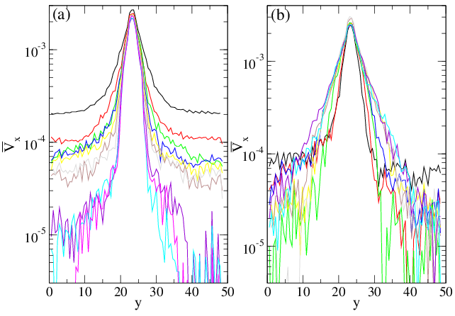
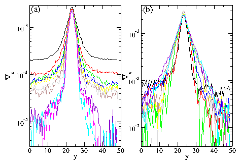
Velocity profiles ―Vx vs y for bidisperse samples with
q1/q2=1.8
at Fd=0.024.
(a) dp=2a and
Np = 0, 4, 6, 8, 10, 12, 14, 16, 18, and 20,
from top center to bottom center.
(b) Np = 10 and
dp=2a, 4a, 6a, 8a, 10a, 12a, 14a, 16a, and 18a,
from bottom center to top center.
Figure 13:
(Color online)
Velocity profiles ―Vx vs y for bidisperse samples with
q1/q2=1.8
at Fd=0.024.
(a) dp=2a and
Np = 0, 4, 6, 8, 10, 12, 14, 16, 18, and 20,
from top center to bottom center.
(b) Np = 10 and
dp=2a, 4a, 6a, 8a, 10a, 12a, 14a, 16a, and 18a,
from bottom center to top center.
|