Physical Review E 83, 041501 (2011)

Anisotropic Sliding Dynamics, Peak Effect, and Metastability in Stripe Systems

C. J. Olson Reichhardt, C. Reichhardt, and A.R. Bishop

Theoretical Division, Los Alamos National Laboratory, Los Alamos, New Mexico 87545

(Received 3 November 2010; published 1 April 2011)

A variety of soft and hard condensed matter systems are known to form stripe patterns. Here we use numerical simulations to analyze how such stripe states depin and slide when interacting with a random substrate and with driving in different directions with respect to the orientation of the stripes. Depending on the strength and density of the substrate disorder, we find that there can be pronounced anisotropy in the transport produced by different dynamical flow phases. We also find a disorder-induced "peak effect" similar to that observed for superconducting vortex systems, which is marked by a transition from elastic depinning to a state where the stripe structure fragments or partially disorders at depinning. Under the sudden application of a driving force, we observe pronounced metastability effects similar to those found near the order-disorder transition associated with the peak effect regime for three-dimensional superconducting vortices. The characteristic transient time required for the system to reach a steady state diverges in the region where the flow changes from elastic to disordered. We also find that anisotropy of the flow persists in the presence of thermal disorder when thermally-induced particle hopping along the stripes dominates. The thermal effects can wash out the effects of the quenched disorder, leading to a thermally-induced stripe state. We map out the dynamical phase diagram for this system, and discuss how our results could be explored in electron liquid crystal systems, type-1.5 superconductors, and pattern-forming colloidal assemblies.
I. INTRODUCTION
II. SIMULATION
III. PULSE MEASUREMENTS AND METASTABILITY FOR STRONG DISORDER
A. Transient Times
B. Pulse Measurements for Weak Disorder
IV. CONTINUOUS FORCE SWEEP MEASUREMENTS
A. Strong Disorder
B. Pinning Strength Dependence and Peak Effect
C. Dynamic Phase Diagram
D. Changing Disorder Density and Radius
V. VELOCITY FLUCTUATIONS
VI. THERMAL EFFECTS
A. Thermally Induced Ordering
VII. SUMMARY
References

I.  INTRODUCTION

Stripe formation occurs in a wide variety of soft [1,2,3,4,5,6,7,8,9,10] and hard [11,12,13,14,15,16,17] condensed matter systems. These stripe patterns are often a consequence of some form of effective competing or multiple length scales in the pairwise interactions between the particles [1,3,4,5,6,9,10,14,18,15,16]. For soft condensed matter, pattern formation can occur when the particles experience intermediate range repulsion and short range attraction, such as in certain types of colloidal systems [6,9]. In addition to stripe phases, numerous other patterns can appear as a function of density, temperature, or particle interaction strength, including bubble, clump, and uniform crystalline phases [1,3,4,5,14,10,17,19]. The competing interactions responsible for the stripe formation may be produced by particles that have both a short range attraction and a long range repulsion [14,18,19,10]; however, systems with only repulsive interactions can also exhibit stripe phases [4,5,7,8] provided that there are at least two length scales in the interaction potential. Typically, as the density increases, the system progresses from a low density clump phase to an intermediate density stripe phase, and then to a higher density bubble phase where organized voids appear in the system; finally, at the highest densities, the particles form a uniform crystal state [4,8,9,19]. In two-dimensional (2D) systems of finite size, a stripe phase containing oriented stripes is often observed [4,5,19]; however, for larger systems, the strong degeneracy in the stripe ground state orientation can produce a labyrinth pattern composed of many different stripe orientations [3,4,8,20]. The presence of any type of bias produced by the boundaries, a substrate, or an external drive such as a shear breaks the symmetry of the stripe ground state and causes the stripes to align in a single direction [20,21,9].
In addition to soft matter systems, there is growing evidence that stripe and bubble phases occur in hard condensed matter systems such as 2D electrons in the quantum Hall regime [17,22,23] and charge ordering in high temperature superconductors [11,12,13,14,15,16]. Evidence for stripe phases in two-dimensional electron gas (2DEG) systems includes anisotropic transport curves which have been interpreted as indicating that the stripes have a single preferred orientation [22,23,24,25]. If the stripes take the form of a charge ordered state, the transport anisotropy implies that the stripes can slide more easily when the drive is applied parallel to the stripes than when it is applied perpendicular to them. The alignment of the stripes in the 2DEG systems may be due to small intrinsic biases that form during sample growth [26]. There have also been recent 2DEG experiments that show that dc drives or other external driving can dynamically orient the stripes under certain conditions [27,28]. Other recent experiments have shown that the stripe direction can be controlled with a strain, making it possible to alter the anisotropy with a strain field [29]. Transport experiments in 2DEGs have revealed sharp conduction thresholds, a series of intricate jumps in the current versus resistance curves, pronounced hysteresis, and changes in the conduction noise, suggesting that these systems are undergoing depinning transitions and dynamic changes in the sliding dynamics [30,31,27]. Additional evidence for charge ordered states in 2DEGs has come from resonance measurements [32,33].
Another recently described system where stripe patterns occur is in "type-1.5" superconductors, predicted to appear in two-band superconductors such as MgB2 [34]. In a type-II superconductor under a magnetic field, the flux in the sample takes the form of quantized vortices which organize into a uniform triangular lattice as a result of their repulsive interactions. In contrast, in type-1.5 superconductors, the vortices have both an attractive and a repulsive component to their interactions [34,35], which in principle will lead to the formation of clumps and stripes. Experiments in the two-band superconductor systems have revealed evidence for disordered clump-like vortex structures; however, strong pinning in the samples probably prevents the detection of ordered patterned structures [34].
In the 2D electron systems and the type-1.5 superconductors, the interplay between the disorder in the sample and an external drive should produce very rich dynamics with different types of depinning transitions and sliding states. It should also be possible to subject stripe-forming soft matter systems to both an external drive and quenched disorder. Experiments have already been conducted on the depinning of purely repulsive colloids interacting with quenched disorder [36]. Similar experiments could be performed with colloidal systems that have interactions which lead to stripe formation. The work we describe here is also relevant to systems exhibiting anisotropic sliding friction due to the formation of stripe-like surface ordering [37]. To address how stripe-forming systems behave in the presence of both driving and quenched disorder, we simulate a collection of particles driven over randomly placed attractive pinning sites and interacting with a long range repulsion and a short range attraction [21,14,19]. We show that when the stripes have a specific orientation, a number of distinct sliding states can occur which have distinct anisotropic transport signatures, including a peak in the anisotropy produced when the dynamics is plastic for driving transverse to the stripes but elastic for driving along the stripes.
In our previous work, we have examined the depinning and sliding of disordered bubble, clump, and stripe phases, and found that for a fixed pinning density, the stripe phase has the highest depinning threshold [21,14]. In this case, the stripes did not have a single orientation but instead formed a disordered labyrinth pattern. When plastic depinning occurred, it was possible to induce a dynamical reordering transition into a stripe state aligned with the driving direction [21]. We also found that the dynamically induced reorientation strongly depends on the strength of the quenched disorder. Only for sufficiently strong quenched disorder are there enough plastic distortions to permit the formation of the oriented stripes [14]. When the pinning is weak, the labyrinth structures depin elastically without any distortions and the aligned stripes never form.
Here we analyze the transition from elastic to plastic depinning and show that for some parameters, the stripe system exhibits a peak effect phenomenon similar to that observed at the transition from elastic to plastic depinning in vortex matter. The vortex peak effect is associated with a sharp increase in the depinning force as well as changes in the transport curves [38,39,40,41]. We show that the peak effect in the stripe system can occur for driving in either direction and that it is possible to have a peak effect for one direction of drive but not the other. In previous work, we showed that there is a broad maximum in the depinning force for the stripe phase as a function of the strength of the attractive term. In this work, we study the peak effect in the stripe phase as a function of disorder and find that it occurs as a sharp, first-order-like transition which is similar to the peak effect observed in superconductors.
In this work we explicitly focus on the case where the stripes are already in an aligned state rather than in a disordered labyrinth phase. This permits us to apply a drive in two well-defined directions, along and perpendicular to the stripes, and to compare the anisotropic response for different strengths of quenched disorder. As noted previously, many of the 2DEG stripe systems appear to contain oriented stripes. To our knowledge the depinning and sliding dynamics of an oriented stripe system has not previously been numerically studied. We find several new types of sliding phases that do not appear for sliding dynamics in isotropic systems such as vortices [42,43,44,45,46,47,48], colloids [40], sliding charge density waves [49], or sliding Wigner crystals [50]. For example, we find several different types of plastic stripe flow. In one state, individual structures slide past stationary stripes; in another state, the stripe structure remains intact but a portion of the particles within the stripes are pinned while other particles flow past in one-dimensional (1D) channels. For strong disorder the stripe structure breaks apart and the flow is similar to the plastic flow observed in isotropic vortex systems [44,45,48]. We also find that the extent to which the stripes reorient is strongly sweep rate dependent. This affects measurements of the depinning thresholds and features in the transport curves.
The paper is organized as follows. In Section II we describe our simulation method. In Section III we employ pulse drive measurements to study metastable and transient behavior of the system. Section III A demonstrates the use of a pulse drive technique to measure transient times as a function of driving force in a system with strong pinning, while in Section III B we show observations of elastic depinning using the pulsed drive. Our careful characterization of the transient behavior permits us to turn to continuously swept drives in Section IV, where we make all measurements at each drive increment in the steady state regime and exclude all transient behavior. Section IV A shows that applying a swept drive to a sample with strong pinning produces plastic flow that is able to erase some memory of the initial state. Section IV B details the peak effect that appears at the transition from ordered to disordered stripe flow. We provide dynamical phase diagrams for swept drives applied along and transverse to the stripes in Section IV C, and consider the effects of changing disorder density and radius on these phases in Section IV D. Section V describes the velocity noise that occurs near the depinning transition. In Section VI we study the effects of temperature, including a thermally induced ordering transition which is illustrated in Section VI A. We conclude with a summary in Section VII.
Fig1.png
Figure 1: The particle positions (black dots) for a system with competing long-range repulsion and short-range attraction. For this density of ρ = 0.36 we obtain a stripe state with the stripes aligned along the y-direction. The external drives are applied either along the stripe direction, FyD, or perpendicular to the stripes, FxD.

II.  SIMULATION

In Fig. 1 we show a snapshot of our system containing stripes oriented in the y-direction. The easy driving direction is along y, parallel to the stripes, while the hard driving direction is along x, perpendicular to the stripe pattern. Our simulation box has periodic boundary conditions with sides Ly=L and Lx=1.097L. We consider N=380 particles with a density given by ρ = N/(LxLy). Here we fix ρ = 0.36. The particles interact with a long range Coulomb repulsion and a short range exponential attraction. The resulting interaction potential is repulsive at very short ranges due to the Coulomb term, attractive at intermediate range, and repulsive at long range. The dynamics of the particles are determined by integrating the following equation of motion:
η d Ri

dt
= − Ni

ji 
V(Rij) + FPi + FDCi + FTi .
(1)
Here Ri is the position of particle i and we take η = 1.
The first term on the right hand side of Eq. (1) is the particle-particle interaction potential
V(Rij) = 1

Rij
Bexp(−κ Rij)
(2)
with Rij = |RiRj|, B=2.0, and κ = 1.0. To avoid the divergence from the Coulomb term at small Rij we place a constant-force cutoff at Rij < 0.1. The Coulomb term does not permit a long range interaction cutoff so for computational efficiency we employ a Lekner summation method to calculate the long range Coulomb force [51]. The second term of the interaction potential is a phenomenological short range attractive interaction.
The second term on the right in Eq. (1) is the force from the quenched disorder, modeled as Np non-overlapping randomly placed parabolic pinning sites with density ρp=Np/(LxLy) and with
FPi = Np

k=1 
(Fp/Rp)Rik(p)Θ(RpRik(p))
^
R
 
(p)
ik 
.
(3)
Here, Rk(p) is the location of pinning site k, Rp is the pinning radius which is set to Rp=0.2 unless otherwise noted, Fp is the maximum force from a pinning site, Rik(p)=|RiRk(p)|, Rik(p) = (RiRk(p))/Rik(p), and Θ is the Heaviside step function. We average our results over several realizations of the quenched disorder when we construct the phase diagrams.
The force FDCi in Eq. 1 arises from an external dc drive applied unidirectionally to all the particles in either the y or x direction, FDCi = FDyy or FDCi = FDxx. We measure the depinning threshold and transport curves for each driving direction by summing over the velocities of the particles, 〈Vα〉 = ∑Ni vi·α with α = x,y.
The final term on the right hand side of Eq. (1) represents the forces from randomly distributed thermal kicks with the following properties: 〈FTi(t)〉 = 0 and 〈FTi(t)FTj(t)〉 = 2ηkBTδijδ(tt), where kB is the Boltzmann constant. In previous equilibrium studies of this system, we identified the densities at which different clump, stripe, and bubble phases occur [52]. Here we work at ρ = 0.36 corresponding to the case of stripes containing approximately three particles per row as shown in Fig. 1. The initial particle positions were obtained from a very slow simulated annealing from a high T to T = 0.0. The stripes align in the y-direction during the anneal, and the pinning potential is not applied until after the annealing process is completed.

III.  PULSE MEASUREMENTS AND METASTABILITY FOR STRONG DISORDER

We first examine the dynamical response when different strengths of external drive are suddenly applied to the system. Pulse measurements have been used extensively to characterize the plastic depinning dynamics of vortex systems [53] but have not to our knowledge been applied previously to study the depinning dynamics of stripe-forming systems. When the external drive is slowly increased from zero, the system passes through several different dynamical phases. In contrast, for the sudden pulse drive, the system can pass directly from a pinned state to a sliding state, and an ordered moving state may appear that cannot be reached by slowly increasing the driving force. For strong pinning, the stripe structure breaks up or fragments near depinning, and the anisotropy of the two driving directions is reduced for a slow ramp of the driving force; however, for the pulse measurements, a pronounced anisotropy can be preserved.
Fig2.png
Figure 2: (a) The average steady state velocity 〈Vy〉 vs FyD for pulse driving in the y-direction. We use the same parameters as in Fig. 1 with Fp=0.9 and ρp=0.38. Here the drive is suddenly increased from zero to FD and the system settles into a steady state after a transient time τ. (b) The corresponding dVy〉/dFyD, with a sharp peak indicating the transition to a moving stripe phase for FyD ≥ 0.165. (c) 〈Vx〉 vs FxD for the same system. (d) The corresponding dVx〉/dFxD vs FxD showing a sharp peak at the transition to a perpendicularly translating stripe state.
Fig3.png
Figure 3: The particle positions (black dots) and particle trajectories (black lines) for the system in Fig. 2(a,b) for pulse driving in the y-direction. The particle trajectories are traced over equal times in panels (a), (c), and (e). (a) At FyD = 0.05 there is a filamentary flow pattern along the stripes. (b) A snapshot of only the particle positions from (a) shows that the stripe structure is partially preserved. (c) At FyD = 0.125, fluctuating plastic flow occurs in which channels of moving particles intertwine and mix while other particles remain pinned. (d) The particle positions only for the system in (c) indicate that the stripe structures are completely disordered. (e) At FyD = 0.2, above the peak in dVy〉/dFyD shown in Fig. 2(b), all the particles are moving in an ordered stripe phase. (f) A plot of only the particle positions from (e) shows the ordered stripes.
We conduct a series of pulse drive simulations at Fp = 0.9 and ρp = 0.38. For these parameters, slow driving ramps would produce a breakup of the stripe structure for driving in either the x or y direction. After we apply the pulse drive, the system typically passes through a transient state and the velocity relaxes to a steady state value after a characteristic time τ. We construct a pulsed-drive velocity-force curve by plotting the average steady state velocity 〈V〉 versus the magnitude of the pulse drive FD. This is shown in Fig. 2(a) and Fig. 2(c) for driving along y and x, respectively. For driving in the easy or y-direction, the critical force Fyc is lower than for driving in the hard or x-direction.
There is a sharp jump to a higher value of 〈Vy〉 just above FDy = 0.165 in Fig. 2(a). For FDy < 0.165, the pinned stripe state undergoes plastic distortion when it moves, but for FDy ≥ 0.165, the pinned stripe is able to depin directly into an ordered moving stripe state, resulting in the jump in mobility. An example of the ordered motion is shown in Fig. 3(e) and Fig. 3(f) for FDy = 0.2. For FyD < 0.165, the stripe structures are partially destroyed when plastic flow occurs at depinning. For weakly plastic flow, the moving stripes persist transiently for a period of time before breaking apart and repinning, as in Fig. 3(a) and Fig. 3(b) at FyD=0.05. In contrast, the stripes are disordered in the strongly fluctuating plastic flow phase when a portion of the particles are pinned while other particles are mobile, as illustrated in Fig. 3(c) and Fig. 3(d) for FDy = 0.125. The transition from the disordered plastic flow regime to the ordered moving stripe regime appears as a pronounced peak in dVy〉/dFyD at FyD=0.165, as shown in Fig. 2(b).
Fig4.png
Figure 4: (Color online) 
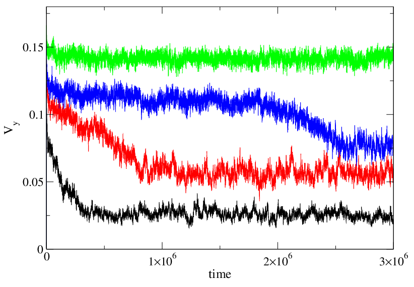
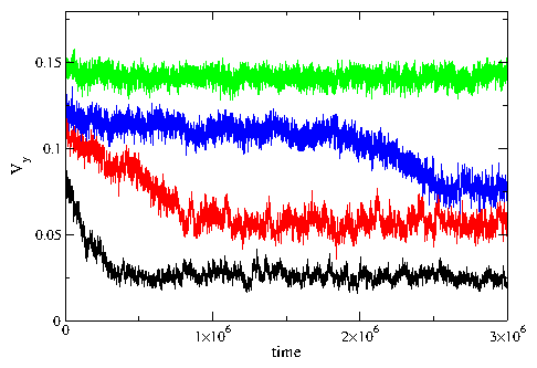
The velocity Vy in the y-direction averaged over every 200 simulation time steps vs time in simulation time steps for pulse drives of FyD = 0.11, 0.125, 0.15, and 0.17, from bottom to top. In the lower three curves, which fall in the strongly fluctuating plastic flow regime, the transition from a higher to a lower velocity occurs when the ordered stripe structure breaks apart, 
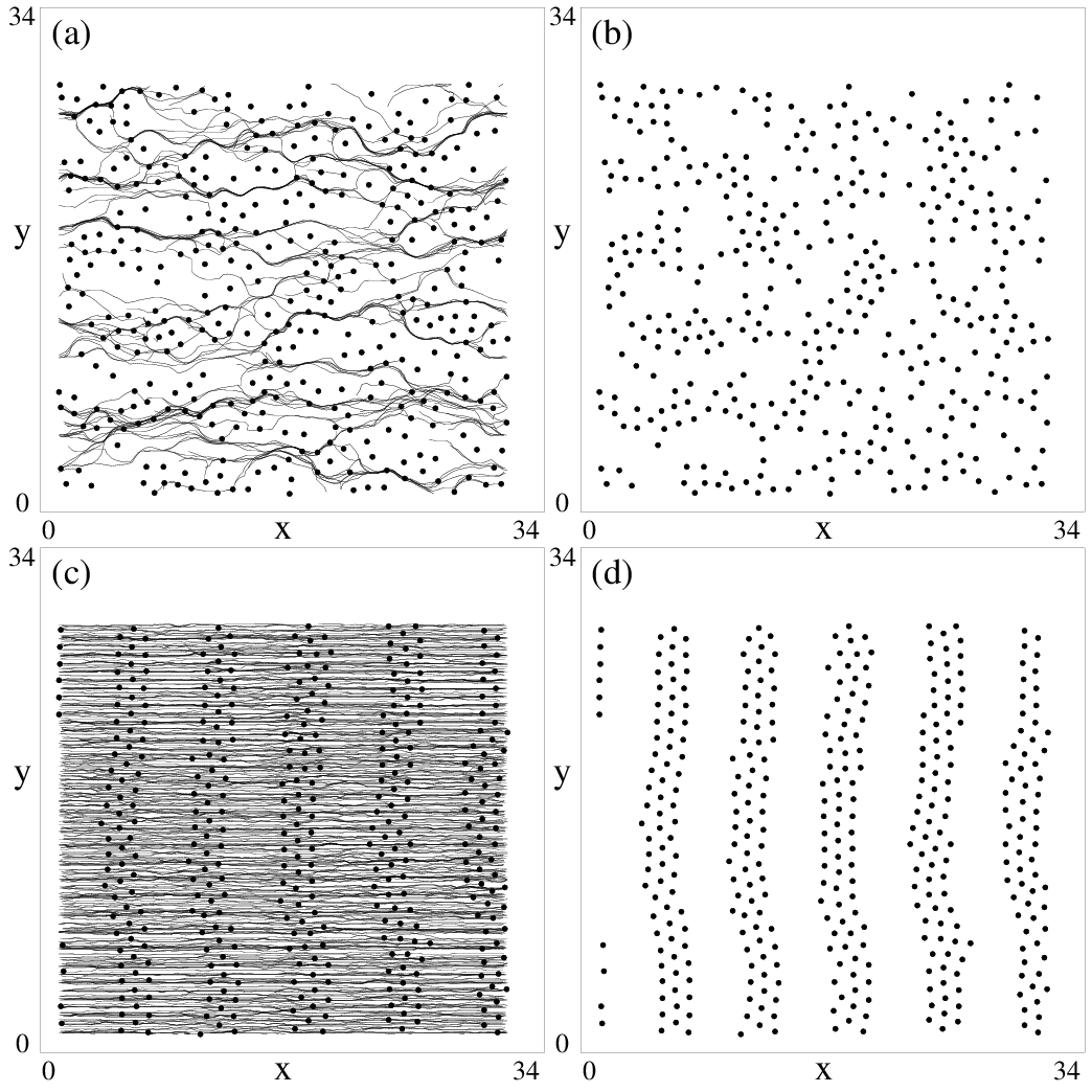
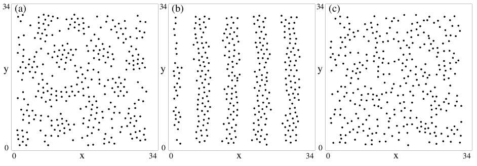
such as when the structure seen in Fig. 3(f) turns into a fragmented structure of the type shown in Fig. 3(d). The upper curve is at a drive above the transition to the moving ordered stripe regime.
For the strongly fluctuating plastic flow regime found for 0.1 < FyD < 0.165, the initial transient motion consists of an elastically moving stripe state in which all the particles are moving. To characterize the time τ required before the system reaches a steady state after application of a pulse drive, we analyze the time series of Vy such as those plotted in Fig. 4 for FyD = 0.11, 0.125, 0.15, and 0.17, where each point is averaged over 200 simulation time steps. The system starts with a higher value of Vy which persists for a time that increases with increasing FyD before dropping to the lower steady state value of Vy. The initial motion associated with the higher value of Vy is a metastable moving ordered stripe. After the transient time τ, the stripe breaks apart and a portion of the particles become pinned, producing the drop to the lower value of Vy. The particle positions shown in Fig. 3(d) at FDy = 0.125 are illustrated at a point in time after the transient ordered stripe state broke apart. In the strongly fluctuating plastic flow regime, transverse diffusion of the particles can occur in which the particles can wander from one stripe to another along the x direction. The nature of this non-thermal diffusion, such as whether it is normal or anomalous, will be the subject of a future study.
For FyD ≥ 0.165, the system remains in the ordered moving stripe state within the entire simulation time window, which includes simulations ten times longer than shown in Fig. 4. For FyD < 0.165, the transient time τ during which the metastable ordered moving stripe exists increases with increasing FyD. It is possible that after extremely long times, even for FDy ≥ 0.165 the stripe state could break apart, resulting in a shift of the peak in dVy〉/dFyD to higher FyD. Figure 2(b) shows that there is a linear increase in dVy〉/dFyD for 0.1 < FyD < 0.16, below the large peak. Within this range of FyD, the steady state flow is strongly fluctuating as shown in Fig. 3(c) and Fig. 3(d). For 0.04 < FyD < 0.1, the 〈Vy〉 versus FDy curve increases very slowly above the depinning transition, as also indicated by the small value of dVy〉/dFDy in Fig. 2(b). In this range of FyD, the flow is still plastic and a portion of the particles remain immobile while others flow past; however, the character of the plastic flow differs from the strongly fluctuating flow found for 0.1 < FyD < 0.16. The low drive plastic flow takes the form of filamentary flow along the stripes, as illustrated in Fig. 3(a) for FyD = 0.05 where one river of particles flows along the stripe. Figure 3(b) shows that the particles still retain much of the stripe structure, in contrast to the strongly fluctuating flow illustrated in Fig. 3(d) where the stripe structure is nearly lost. Another difference is that the plastic flow in Fig. 3(c) involves a significant transverse diffusion of particles in the x-direction, so that over time the particles can mix throughout the system. For the low drive plastic flow in Fig. 3(a), there are some early time particle jumps transverse to the drive from one stripe to another; however, these events vanish in the long time limit and there is no steady state diffusion in the x-direction, even though the shape of the filamentary flow within one stripe may change slightly over time.
Fig5.png
Figure 5: The particle positions (black dots) and particle trajectories (black lines) for the system in Fig. 2(c,d) for pulse driving in the x-direction. The particle trajectories are traced over equal times in panels (a) and (c). (a) At FxD = 0.125, fluctuating plastic flow occurs in which channels of moving particles intertwine and mix while other particles remain pinned. (b) The particle positions only for the system in (a) indicate that the stripe structures are completely disordered. (c) At FxD = 0.23, above the peak in dVx〉/dFxD shown in Fig. 2(d), all the particles are moving in an ordered transverse moving stripe phase. (d) A plot of only the particle positions from (c) shows the ordered stripes.
In Fig. 2(c) we plot 〈Vx〉 versus FxD for the same system in Fig. 2(a), while the corresponding dVx〉/dFxD appears in Fig. 2(d). For the x-direction pulse drive, we do not find any regime where the stripes can dynamically reorient and align themselves in the x direction. Instead, the system passes directly into a moving stripe phase in which the stripe orientation remains perpendicular to the direction of stripe motion, as shown in Fig. 5(c,d). The transition into the sliding stripe phase occurs at the peak in dVx〉/dFxD shown in Fig.2(d) at FxD = 0.224. This peak falls at a higher value of FxD than the value of FyD of the peak in Fig. 2(b). This is because stripes moving perpendicular to their orientation are much more susceptible to breaking apart than stripes moving parallel to their orientation. A higher pulse driving force reduces the effectiveness of the pinning and reduces the tendency for plastic flow, so a stripe moving perpendicular to its orientation is stabilized at a higher drive than a stripe moving parallel to its orientation for the same pinning strength.
Figure 2(d) also shows a smaller maximum in dVx〉/dFxD near FxD = 0.135, corresponding to a change in the character of the plastic flow. For 0.135 ≤ FxD < 0.224, the steady state flow is dominated by strong plastic rearrangements where the stripe structure completely breaks apart, as illustrated in Fig. 5(a,b). In contrast, for 0.06 < FxD < 0.135, the flow is more filamentary and is composed of a small number of slowly changing channels. For 0.17 < FxD < 0.22, we also find a metastable effect similar to that shown in Fig. 4 for driving in the y-direction. An ordered stripe can slide perpendicular to the direction of the stripe orientation for a period of time which increases with increasing FxD before the stripe breaks apart.
In Fig. 2(a) and (c), for 0.15 < Fx,yD < 0.224, the velocity is higher for driving along the easy y direction. In contrast, for 0.08 < Fx,yD < 0.15, 〈Vy〉 falls below 〈Vx〉. This occurs because the pulse drive measurements preserve some of the initial structure of the oriented stripes. In the low drive regime 0.08 < Fx,yD < 0.15, much of the flow is filamentary. For driving along the stripe, FDy, the filamentary flow settles quickly into a few nonfluctuating channels, while for driving against the stripe, FxD, the filamentary flow forms fluctuating plastic channels which generally have large velocity pulses, producing a larger average velocity 〈Vx〉. For 0.025 < Fx,yD < 0.04, anisotropy appears due to the differing critical depinning forces in the two directions; here, flow only occurs in the y-direction but is absent in the x-direction.

A.  Transient Times

We next analyze in detail the time required for the system to achieve steady state flow under a pulse drive. This time grows rapidly near the transition between the disordered and ordered flow states, as shown in Fig. 4. Recent experiments and simulations of periodically sheared particle assemblies under suddenly applied shear have shown evidence for a diverging time to reach a steady state upon approaching a dynamic phase transition [54]. Recent simulations of the plastic depinning of repulsively interacting particles also revealed that the transient time to reach a steady state under a pulsed drive diverges as a power law as the depinning transition is approached from either side [55]. This suggests that analyzing the transient time required to reach a steady state can be a useful diagnostic for probing changes in dynamical states.
Fig6.png
Figure 6: The time τ in simulation time steps required for the system to reach a steady state velocity after an applied pulse drive for the system in Fig. 2. (a) τ vs FyD for driving in the y-direction. The first peak at FyD=0.04 corresponds to the depinning transition, the second peak centered at FyD=0.1 appears at the transition from the filamentary flow illustrated in Fig. 3(a,b) to the fluctuating flow state shown in Fig. 3(c,d), and the third peak at FyD=0.165 is associated with the transition to a moving ordered stripe state. (b) τ vs FxD for driving in the x-direction.
In Fig. 6(a) we plot the transient time τ taken by the system in Fig. 2(a) to reach a steady state after the application of a pulse drive in the y-direction. For FyD < 0.04, below the critical depinning force Fyc, there is still a finite transient time during which the system organizes into a pinned state. The time required to reach the pinned state increases as Fyc is approached from below, while the time required to reach a steady moving state increases as Fyc is approached from above. For FyD ≥ 0.165, when the system passes directly into a moving ordered stripe state, the steady state velocity is reached very quickly and τ is very small. In the region 0.1 < FyD < 0.165, the system depins into a metastable moving ordered stripe state that breaks apart after a time τ as shown in Fig. 4. As FyD approaches FyD=0.165 from below, τ increases since it takes increasingly longer times to trigger the instability that results in the fragmentation of the stripes. The rapid increase of τ suggests that τ may diverge at the transition to the moving stripe phase; however, our results are not accurate enough to establish whether this divergence has a power law form. We find that the peak in τ at FyD = 0.165 is asymmetric. In comparison, the dynamic phase transitions studied in the shearing systems produced symmetric diverging time scales on both sides of the transition [54,55]. Fig. 6(a) also shows a peak in τ centered near FyD=0.09, which corresponds to the location of the change in slope of 〈Vy〉 versus FyD in Fig. 2(a). At this drive, there is a change from the filamentary plastic flow channels shown in Fig. 3(a,b) to the rapidly fluctuating disordered plastic flow channels shown in Fig. 3(c,d). The fact that τ also increases in this region is further evidence that there can be dynamical phase changes even within the plastic flow regime. Finally, there is another peak in τ near FyD = 0.04 at the depinning transition. These results show that peaks in the transient time can be used to detect changes in the flow characteristics of these systems.
In Fig. 6(b) we plot τ for pulse driving in the x-direction. Near FxD=0.225 there is a peak in τ associated with the transition to the moving perpendicular stripe phase. Within the range 0.21 < FxD ≤ 0.225, where the value of τ is locally enhanced, the system forms a metastable state of stripes moving perpendicular to their length. Eventually, the stripes break apart, and the time required for this to occur increases with increasing FxD until for high enough FxD the moving perpendicular stripe structure becomes stable rather than metastable and τ drops back to a small value. The peak in τ at FDx=0.225 in Fig. 6(b) is similar to the peak found for driving in the y-direction in Fig. 6(a) near FyD = 0.165. Figure 6(b) shows that there is another peak in τ centered at FxD = 0.06 corresponding to the transition from filamentary plastic flow to strongly disordered plastic flow. Overall, the transient times for driving in the x-direction are smaller than for driving in the y-direction. For driving along the y-direction, plastic flow channels can form which do not distort the aligned stripe pattern, permitting the system to remain in a metastable state for longer times before falling into the disordered steady state stripe structure. For driving along the x-direction, the stripe structure is more strongly disordered even at lower drives, so the system is closer to the disordered steady state stripe structure from the beginning and spends a shorter amount of time in the metastable state.
Fig7.png
Figure 7: (Color online) Solid line: Vy vs time for FyD = 0.085 for the system from Fig. 2, showing the decay of the system into the filamentary plastic flow state. Dashed line: a power law fit to Vy(t) ∝ t−α with α = 0.35 ±0.05.
The filamentary plastic flow regime that appears for 0.04 < FyD < 0.1 is associated with large values of τ as shown in Fig. 6(a). In this regime, the time decay of Vy to its steady state value differs from the decay in the strongly fluctuating plastic flow regime shown in Fig. 4, where Vy remained roughly constant before dropping relatively rapidly to a lower value. Instead, in the filamentary regime Vy follows a continuous stretched exponential form or power law, as illustrated in Fig. 7 for FDy=0.085. The dashed line is a power law fit performed for t < τ to Vyt−α with α = 0.35 ±0.05. For t > τ, Vy ceases to decay and reaches a steady state. We find an equally good fit of the decaying portion of the curve to a stretched exponential form. The exponents from the fits do not appear to be universal and change when we take measurements from the other plastic flow regimes. We note that in other dynamical regions, the velocity decays exponentially to a steady state. Our results indicate that within the filamentary plastic flow phases, very long transient times can occur.
The order-disorder transition at FyD=0.165 between the lower drive strongly fluctuating plastic flow phase shown in Fig. 3(d) and the higher drive moving ordered stripe phase shown in Fig. 3(f) exhibits metastability and has a diverging time scale only on the low drive side of the transition, as indicated in Fig. 6(a). These features strongly suggest that this transition is first order in nature and that the details of the transition are strongly affected by the initial conditions of the moving state. For example, it is possible to obtain a reversed metastability by starting the system in a disordered configuration and applying a pulse drive FyD > 0.165. In this case, the moving system remains disordered and travels at a lower velocity until an instability causes the stripe structure to form with a corresponding increase in the velocity. This reversed metastability shows diverging transient times as the transition is approached from above, but has no diverging time scales when the transition is approached from below. The metastability of the ordered and disordered states resembles the superheating or supercooling recently observed for systems with first order phase transitions. Very similar dynamical superheating and supercooling effects were found in superconducting vortex systems in experiments [56] and three-dimensional (3D) simulations [57]. The vortex system undergoes a disorder-induced first order phase transition, and the effective disorder changes when the system is prepared in different states. Computational studies of 2D vortex systems interacting with disorder have shown that there is either a continuous order to disorder transition or a crossover, so hysteresis, superheating and supercooling do not appear. For many stripe forming systems in two dimensions, transitions from ordered to disordered states in equilibrium and in the absence of quenched disorder are first order in nature [4,5]. Our results suggest that the first order nature of the equilibrium transitions persists for some of the transitions between nonequilibrium states.
At the transition between the low drive filamentary plastic flow phase and the higher drive strongly fluctuating plastic flow phase, Fig. 6(a) indicates that there are diverging transient times on both sides of the transition. This behavior is similar to the diverging transient times found for 2D plastic depinning. There is evidence that the plastic depinning is an absorbing phase transition falling in the directed percolation class [55]. Determining whether the depinning of the stripe system or the filamentary plastic flow to strongly fluctuating plastic flow transition are also nonequilibrium phase transitions falling in the directed percolation class is beyond the scope of this work; however, our results suggest that the stripe system may be an ideal system in which to examine the nature of nonequilibrium transitions since it exhibits several different types of flow phases.
Fig8.png
Figure 8: (Color online) (a) 〈Vy〉 vs FyD for a pulse drive system with ρp=0.38 and a lower pinning force of Fp = 0.125. A two step depinning occurs, with uncoupled stripes depinning initially followed by the depinning of coupled stripes. (b) The corresponding dVy〉/dFyD has a double peak indicating the two step depinning process. (c) 〈Vx〉 vs FxD for the same system. Inset: Plot of 〈Vx〉 vs FxDFxc for the data in the main panel with Fxc=0.00345. The dashed line indicates a power law fit with an exponent of β = 0.35. (d) The corresponding dVx〉/dFxD shows a single step elastic depinning of the stripes.
Fig9.png
Figure 9: (Color online) A combined plot of 〈Vx〉 vs FDx (dark line) and 〈Vy〉 vs FDy (light line) for the system in Fig. 8 with Fp=0.125 highlighting the transport anisotropy. Inset: The particle positions (dots) and trajectories (lines) for the system in Fig. 8(a) in the decoupled stripe regime at FyD=0.0025 where a portion of the stripes are moving while others are pinned.

B.  Pulse Measurements for Weak Disorder

We next consider pulse drive measurements for a system with the same pinning density ρp=0.38 but with a weaker disorder strength of Fp=0.125. In Fig. 8(c) we plot 〈Vx〉 versus FxD and in Fig. 8(d) we show the corresponding dVx〉/dFxD. For this value of Fp, the stripe structure remains ordered. The single step depinning for x-direction driving is elastic and has 〈Vx〉 ∝ (FxDFxc)β, with β = 0.35, as shown in the inset of Fig. 8(c). This is followed by a crossover to 〈Vx〉 ∝ FxD at higher drives. The behavior agrees well with the depinning of a harmonic elastic string driven over a random substrate, where an exponent β = 0.33 is observed [58]. For driving in the y-direction, as shown in Fig. 8(a), 〈Vy〉 versus FDy indicates that a two step depinning process occurs. The initial depinning involves the flow of individual stripes, while other stripes remain pinned or move at different velocities, as illustrated in the inset of Fig. 9 for FyD=0.0025. At higher drives, the remaining stripes depin and become coupled to the other moving stripes, resulting in an elastic flow. The two peaks in dVy〉/dFyD shown in Fig. 8(b) fall at the locations of the two depinning transitions. A similar type of two step, layered depinning transition was predicted for anisotropic charge density wave (CDW) systems, where CDWs first depin separately and flow independently from one layer to the next, and then recouple at higher drives [59]. Mean field models also predict that layered systems should show a coupling-decoupling transition [60,61], while two-layer models predict that coexistence of moving and pinned phases should occur in 2D systems [62]. In the main panel of Fig. 9, we plot 〈Vx〉 versus FxD and 〈Vy〉 versus FyD together in order to highlight the transport anisotropy which disappears for Fx,yD > 0.04 when fully elastic flow is established. The transient times τ for the Fp=0.125 system are much shorter than those in the Fp=0.9 system, where plastic depinning occurred. We find an increase in τ just below each depinning transition in the Fp=0.125 system for both x and y direction driving. For x-direction driving, there is a single peak in τ below the depinning threshold which is associated with a small amount of roughening of the stripe structure that occurs just before depinning. Above each depinning transition in the weak pinning system, τ is extremely small. For y-direction driving, the peak in τ is broader within the sliding plastic flow phase found below the second depinning transition. In systems with even weaker pinning, Fp < 0.05, the depinning is elastic for both driving directions and the transport anisotropy is significantly reduced.
Fig10.png
Figure 10: (Color online) A combined plot of 〈Vx〉 vs FxD (dark line) and 〈Vy〉 vs FyD (lighter line) for a system with Fp=0.9 and the same parameters as in Fig. 2 but with a continuously swept drive. There are several steps in 〈Vy〉 that appear below the drive Fx,yD=0.32 at which the two curves meet. Inset: A blow-up of the region near Fx,yD = 0.24 shows a crossing of the 〈Vx〉 and 〈Vy〉 curves, indicating that 〈Vy〉 has a smaller slope and that therefore fewer particles are moving for driving in the y-direction than for driving in the x-direction. The crossing of 〈Vx〉 and 〈Vy〉 does not occur for the pulse drive measurements shown in Fig. 2.
Fig11.png
Figure 11: (a) Image of particle positions in the reordered phase at FyD=0.27 in the swept drive system from Fig. 10. In addition to the stripe structure, there are some scattered particles pinned between the stripes. (b) Image of particle positions in the reordered phase at FxD=0.27 in the same system. The stripes have reoriented in the x-direction and there are no pinned particles between the stripes.

IV.  CONTINUOUS FORCE SWEEP MEASUREMENTS

A.  Strong Disorder

We now examine the case where the applied drive is slowly incrementally increased in a single sweep as opposed to the sudden application of the drive discussed in the previous section. We use a driving force increment of ∆FD=0.00025 applied every 25000 simulation time steps in a system with Fp = 0.9 and ρp = 0.38. In Fig. 10 we plot the resulting 〈Vx〉 versus FxD and 〈Vy〉 versus FyD together. Many of the transport features are the same as those shown for the pulse drive in Fig. 2, such as the lower depinning threshold for driving in the y-direction and the anisotropic flow centered near Fx,yD = 0.2. The transition to the flowing stripe state remains sharp for the continuous sweep drive in the y-direction, but for the x-direction driving the state in which the stripes flow perpendicular to their orientation is lost. Instead, the system reorders into a stripe state oriented along the x-direction, as shown in Fig. 11(b) for FxD = 0.27. In the pulse drive system, the perpendicular moving stripe state can be stabilized by dynamical quenching, but for the swept drive, the system passes through an extensive plastic flow phase which destroys any memory of the initial perpendicular stripe orientation.
The inset of Fig. 10 highlights that under the swept drive, a crossing of 〈Vy〉 and 〈Vx〉 occurs near Fx,yD = 0.24. There is no such crossing for the pulse drive, as shown in Fig. 2. The crossing of the curves indicates that although the system is in the moving stripe state for both drive directions, the slope of 〈Vy〉 is smaller than that of 〈Vx〉 in this regime. This is because a fraction of the particles remain pinned for the y-direction drive, while all of the particles are moving for the x-direction drive. When fewer particles are moving, the slope of the velocity-force curve is reduced. Particles are able to remain pinned for the y-direction drive because they can be captured in pinning sites that are sufficiently far away from the neighboring stripes that they experience only repulsion from the particles in the stripes, and are out of the range of the attractive part of the particle-particle interaction potential. This does not happen for the x-direction drive because during the stripe reorientation process, all pinned particles are eventually swept up into a moving stripe. In Fig. 11(a), the reordered stripe phase for FyD = 0.27 contains pinned particles that sit between the stripes rather than flowing with the stripes. In contrast, in the moving stripe phase for a y-direction pulse drive shown in Fig. 3(f), there are no pinned particles between the moving stripes. In the x-direction swept drive moving stripe phase, all of the particles are moving and there are no pinned particles between the moving stripes, as shown in Fig. 11(b) for FxD=0.27. The transition into the moving stripe phase for swept y-direction driving is rapid, as indicated by the jump in 〈Vy〉 at FyD = 0.185 in Fig. 10. For x-direction driving, the reordering transition is more continuous, permitting more meandering of the stripe pattern during the stripe formation process. This allows all of the pinned particles to be attracted gradually into the moving stripe structure.
Once the driving force becomes strong enough, the pinned particles surrounding the moving stripes for the y-direction swept drive depin and join the moving stripe structures. The depinning of the individual particles produces the step features in 〈Vy〉 near FyD = 0.28 in Fig. 10. For drives above the depinning threshold of all of the pinned particles, the velocity response is isotropic, as shown in Fig. 10 for FDx,y > 0.32. Our results indicate that even for pinning strengths strong enough to induce plastic flow and a subsequent reordering of the stripe structure, some memory of the initial ordering of the stripe phase is retained up to relatively large values of the driving force. We note that based on the extended transient behavior found in the plastic flow regimes for the pulse drives, it is possible that if the swept drives were applied with even slower drive increments, the anisotropic response could be lost at lower drives if the system is given more time to slowly mix in the plastic flow state.
Fig12.png
Figure 12: (Color online) A combined plot of 〈Vx〉 vs FxD (dark line) and 〈Vy〉 vs FyD (lighter line) for a system with ρp=0.38, a lower Fp=0.225, and a swept drive. The depinning in the x-direction is accompanied by plastic distortions and the partial breaking apart of the stripe structure. Depinning in the y-direction occurs by the sliding of stripes past one another in a manner similar to that illustrated in the inset of Fig. 9.
Fig13.png
Figure 13: (Color online) (a) The critical depinning forces Fxc (filled circles) and Fyc (open squares) for driving in the x and y-directions, respectively, plotted vs Fp. The sharp jumps in the depinning forces are associated with changes from elastic flow to plastic flow and from plastic flow to sliding ordered flow. (b) The corresponding dFxc/dFp vs Fp (dark line) and dFyc/dFp vs Fp (light line) curves more clearly show the onset of the different depinning phases. (c) The anisotropy ratio R = Fxc/Fyc vs Fp shows that the change in anisotropy can be associated with different depinning regimes.

B.  Pinning Strength Dependence and Peak Effect

When we perform swept drive measurements on a system with the weaker pinning strength of Fp=0.125, we obtain velocity-force curves that are nearly identical to those shown in Fig. 8 for a pulse drive measurement. We attribute this to the lack of plastic flow in the weakly pinned system. Without plastic flow, the stripe structure never breaks apart and memory of the initial stripe orientation is never lost, so the same stripe orientation appears, regardless of whether the drive is slowly swept or suddenly applied. By increasing Fp slightly, we reach a state where the x-direction depinning is plastic and accompanied by the breaking apart of the stripe structure, while the y-direction depinning occurs by the sliding of some of the stripes, with the stripe structure maintained intact. This situation is illustrated in Fig. 12, where we plot 〈Vx〉 versus FxD and 〈Vy〉 versus FyD for a swept drive system with Fp=0.225.
By conducting a series of simulations for varied Fp, we map the anisotropy in the depinning thresholds Fxc and Fyc, as shown in Fig. 13(a). For x-direction driving, Fxc increases monotonically with increasing Fp for 0 < Fp < 0.175. Within this range of Fp, the depinning is elastic and the stripes move perpendicularly to their orientation. Each particle maintains its position in its original stripe. Just above Fp = 0.175, there is a sudden increase in Fxc corresponding to the onset of plastic distortions of the stripe structure at depinning. For driving in the y-direction, Fyc continuously increases with increasing Fp for 0 < Fp < 0.25. Over this range of Fp, the stripes depin elastically and either all depin simultaneously for Fp < 0.05, or depin as individual sliding stripes for 0.05 ≤ Fp < 0.25 via the mechanism illustrated in the inset of Fig. 9. For Fp < 0.05, where our system behaves elastically, we find that Fyc increases approximately quadratically with Fp which is the expected behavior for elastic depinning [63]. Just above Fp = 0.25 there is a sharp increase in Fcy when the stripes begin to depin plastically along individual stripes in the manner shown in Fig. 3(a).
For Fp > 0.4, both Fyc and Fxc begin to saturate, as shown by the anisotropy ratio R=Fcx/Fcy plotted in Fig. 13(c). The saturation arises due to the fact that the number of pinning sites Np is only slightly higher than the number of particles N. As a result, when Fp is large enough, the initial depinning is dominated by interstitially pinned particles. These particles are not trapped by one of the randomly located pins, but are instead held in place by interactions with neighboring pinned particles. The critical force for the depinning of particles trapped by pins increases linearly with increasing Fp, but the critical force for the depinning of interstitially pinned particles is determined only by the particle-particle interaction potential and is not altered by increasing Fp. In a system with a much higher pinning density, every particle would be trapped by a pin and the depinning threshold would show the expected linear increase with increasing Fp.
The sharp increases in the depinning thresholds associated with transitions from elastic to plastic flow or from weakly plastic flow to a more strongly plastic flow resemble the phenomenon observed for depinning of vortices in type-II superconductors, where a peak in the depinning threshold has been connected with the disordering of the vortex lattice [39,64,38,40,41,65,56,57]. In the disordered or plastically flowing systems, the particles can more readily adjust their positions to take advantage of the energy of a randomly located pinning site without paying the large energy cost required to distort an elastic or ordered particle lattice. In studies of 2D vortex systems, as the vortex lattice is softened the system becomes more disordered and the depinning threshold increases continuously, producing a peak effect that is continuous rather than sharp [66]. This may be related to the fact that 2D systems of particles with repulsive long range interactions lack first order melting or disordering transitions. Many 3D vortex systems have a first order transition from an ordered vortex structure to a disordered one, and the peak effect phenomena observed in these systems is very sharp. Even through the stripe system described here is 2D, the pairwise particle interactions are not strictly repulsive. Previous studies in the absence of quenched disorder using the same model produced results that suggest that the thermal melting of the stripe and clump systems is a first order transition. Other 2D studies of stripe-forming systems with competing interactions also find first order melting transitions for many of the phases [4]. These results suggest that the first order peak effect phenomenon found for vortex systems may also generically occur for stripe and pattern forming systems in the presence of quenched disorder. We note that one of the features of the peak effect in superconducting systems is that at fields or temperatures above the sharp increase in the depinning force, the critical current or critical depinning force decreases again. The decrease results from the changes in the penetration depth and coherence length that occur as the system approaches Tc or Hc2. The peak effect itself is associated with a pinning-induced transition from ordered or elastic flow to disordered or plastic flow, which is exactly what we observe in our stripe system.
To further characterize the changes in Fc we plot dFxc/dFp and dFyc/dFp vs Fp in Fig. 13(b). There is a peak in dFxc/dFp near Fp = 0.185 corresponding to the transition from ordered stripe flow to partially plastic flow. A second, much broader peak appears near Fp = 0.35 at the point where the stripes break apart completely. For 0.185 < Fp < 0.35, the stripes driven in the x-direction reorder into a perpendicularly moving stripe state at high FxD in spite of the fact that weakly plastic flow occurs above depinning. For Fp ≥ 0.35, the plasticity at depinning becomes much stronger and the stripes reorder into a parallel moving state at high FxD. For driving in the y-direction we find a single sharp peak in dFyc/dFp near Fp = 0.25 corresponding to the appearance of plastic flow along the stripes. We note that the transition at Fp=0.075 into the pinned-sliding phase illustrated in the inset of Fig. 9 is not associated with any sharp features in dFyc/dFp.
The appearance of different flow phases can also be detected in the plot of the anisotropy ratio R in Fig. 13(c). For example, the peak in R over the range 0.185 < Fp < 0.3 occurs when the flow for x-direction driving is plastic, while the flow for y-direction driving remains elastic in the stripe sliding state. The increase in R at Fp = 0.06 corresponds to the transition from elastic depinning in both directions to elastic depinning for x-direction driving and individual stripe sliding for y-direction driving. For Fp > 0.6, the anisotropy begins to saturate.
Fig14.png
Figure 14: (Color online) Dynamic phase diagrams showing the onset of depinning (lower heavy line) and the onset of the dynamic stripe reordering (upper light line). (a) FxD vs Fp. The dashed line separates the moving perpendicular stripe phase from the dynamically reordered parallel stripe phase. In order for the parallel stripe phase to form, the system must first pass through a strongly fluctuating plastic flow phase. (b) FyD vs Fp. The dashed line indicates the change from sliding stripe plastic flow to plastic flow in which the stripe structure breaks apart.

C.  Dynamic Phase Diagram

By identifying features in the velocity force curves and associating them with different moving states, we construct a dynamic phase diagram for both x and y direction driving. In Fig. 14(a) we plot the phase diagram for FxD vs Fp, indicating the location of the depinning curve and the transition into an ordered stripe state. For Fp < 0.185, the stripes depin elastically into a perpendicular moving stripe state, while for 0.185 ≤ Fp < 0.35, the stripes depin with a small amount of plastic distortion into the same perpendicular moving stripe state. The line in Fig. 14(a) marking the transition from plastic flow to reoriented ordered parallel moving stripes increases roughly linearly with Fp for Fp > 0.4.
In Fig. 14(b) we plot the phase diagram of FyD versus Fp for driving in the y-direction. In this case the stripes are always oriented in the direction of the drive. The range of the plastic flow regime grows with increasing Fp and in general the onset of the moving stripe phase occurs at lower drives than those at which the parallel moving stripes form for x-direction driving. The small dashed line indicates the transition from the plastic flow in which the stripe structure is destroyed for Fp ≥ 0.275 to the state where moving stripes slide past pinned stripes for 0.075 < Fp < 0.275.
The dynamic phase diagram for the stripe system contains a larger number of phases than dynamic phase diagrams observed in systems with purely repulsive particle-particle interactions moving over random disorder. For example, in 2D vortex systems the dynamic phases consist only of a pinned state, a plastic flow state, and a moving partially ordered state, and the transitions between these states are continuous. In the partially ordered moving state, the particles are not fully crystallized but develop a smectic type of ordering and flow in evenly spaced channels aligned with the direction of the drive. The channels of flow may be coupled or partially coupled [42,43,44,45,46]. This is similar to the state we observe in which the stripes reorient in the direction of drive for sufficiently high drive and sufficiently strong pinning. In the stripe system, the stripe reordering transition is more consistent with a first order phase transition rather than the continuous or crossover behavior found for particles with purely repulsive interactions. Studies of driven systems with quenched disorder, where the particle-particle interactions are more complicated than the purely repulsive case, have shown that it is possible to have a coexistence of different moving phases, which is consistent with having first order phase transitions between the moving phases [67].
Fig15.png
Figure 15: (Color online) (a) Fxc (filled circles) and Fyc (open squares) vs ρp for a system with Fp = 0.225 and Rp = 0.3. (b) The corresponding R = Fxc/Fyc vs ρp shows that at large ρp the anisotropy is reduced. (c) Fxc (filled circles) and Fyc (open squares) vs ρp for a system with Fp = 0.7 and Rp=0.3. (d) The corresponding R vs ρp. Here the anisotropy drops nearly to R=1 at high ρp

D.  Changing Disorder Density and Radius

In Fig. 15(a) we plot Fxc and Fyc versus ρp for a system with Fp = 0.225 and Rp=0.3, and in Fig. 15(b) we show the resulting anisotropy ratio R = Fxc/Fyc versus ρp. Here Fxc and Fyc both increase monotonically with increasing ρp. We work with Rp=0.3 rather than Rp=0.2 in order to more easily access the steady state for low values of ρp. Empty pinning sites with smaller Rp are more easily screened by occupied neighboring pinning sites when an unpinned particle is unable to reach the empty pinning site due to the long-range repulsion of the nearby pinned particle. The empty pins can eventually be occupied after a lengthy transient time. We find that the transient times for low ρp are reduced to manageable levels when we take Rp=0.3 instead of Rp=0.2. Fig. 15(b) shows that at low ρp the anisotropy R is strongly reduced and the two depinning curves come together when the depinning becomes elastic for both x and y-direction drives. A similar effect appears in Fig. 13(c) for low Fp, where the onset of elastic depinning for both driving directions results in a reduced value of R. The anisotropy in Fig. 15(b) passes through a maximum near ρp = 0.2 before gradually falling back to 1.0 for increasing ρp. The pinning density plays a more important role in determining the anisotropy of the depinning for pre-formed stripe states than the pinning strength. When the average distance between pinning sites is greater than the inter-stripe distance, depinning for y-direction driving in a system with strong pinning occurs via a combination of plastic flow of particles along some stripes while other stripes remain completely pinned. As a result, Fyc is generally lower than Fxc for the low density, strong pinning limit. This is shown in Fig. 15(c) where we plot Fyc and Fxc versus ρp for Fp = 0.7. For higher values of ρp, the plastic depinning along the stripes for y-direction driving is suppressed and the behavior becomes more isotropic. For systems with small ρp and Fp > 0.35, the anisotropy persists down to much lower values of ρp than shown in Fig. 15(a); however, for ρp > 1.0 the anisotropy vanishes completely.
Fig16.png
Figure 16: (Color online) (a) Fxc (filled circles) and Fyc (open squares) vs Rp for a system with Fp = 0.225 and ρp = 0.38. (b) The ratio R = Fxc/Fyc vs Rp showing that the anisotropy increases with increasing Rp and saturates at high Rp.
We next consider a system with Fp = 0.225 and ρp = 0.38 with varied pinning radius Rp. We plot Fxc and Fyc versus Rp in Fig. 16(a), and the anisotropy ratio R = Fxc/Fyc in Fig. 16(b). Both Fxc and Fyc increase with increasing Rp. For low Rp, Fxc increases faster with increasing Rp than Fyc does, and for high Rp, the anisotropy R saturates.

V.  VELOCITY FLUCTUATIONS

The dynamic phases can also be characterized by measuring the velocity fluctuations. Experiments on stripe forming systems previously demonstrated that narrow band noise, characterized by a periodic noise signal, and broad band noise, which lacks any characteristic frequencies, can occur and showed evidence for transitions between the different types of noise [31,68]. Previous simulations of clump and stripe forming systems showed the presence of a 1/f noise characteristic in the nonlinear portion of the velocity-force curve associated with the fluctuating plastic flow phase. At high drives where the stripes or clumps reorder, the noise becomes white with a weak narrow band or washboard frequency similar to that observed for a driven vortex lattice in the dynamically reordered regime [45].
Fig17.png
Figure 17: (Color online) (a) The time series of Vy for a system with Fp = 0.9, ρp = 0.36, Rp = 0.2, and FyD = 0.04. For these parameters, the particles move in stationary plastic filaments, producing a periodic time-of-flight signal. (b) The power spectrum S(f) of the time series in (a) showing the characteristic peaks from the periodic signal. Here, f is in units of inverse simulation time steps. (c) Time series of Vy for the same system at FyD = 0.12 in the strongly fluctuating plastic flow regime. (d) The corresponding S(f) has a 1/f feature at low frequencies as indicated by the dashed line.
Here we show that the stripe system exhibits many additional noise features near depinning. For y-direction driving near depinning, there can be filamentary plastic flow channels along the stripe with no particle diffusion from stripe to stripe, as shown in Fig. 3(a). Within this filamentary plastic flow regime, it is possible for the particle flow to be limited to one or a small number of individual winding channels which do not change over time and which have a characteristic time-of-flight for crossing the sample. This results in a periodic velocity signal such as that shown in Fig. 17(a) for a system with Fp = 0.9 and FyD = 0.04. Similar periodic filamentary plastic motion has been observed in vortex simulations performed just at depinning. Here one or two stable channels of moving particles form while the rest of the particles are immobile [69]. Evidence for filamentary flow has also been found in vortex experiments, where a series of jumps and dips in the current-voltage curve were interpreted as indicating the opening of individual channels of vortex flow [70]. There are also several simulations of vortex systems showing transitions from narrow band filamentary flow to chaotic flow as the drive is increased [71]. The power spectrum S(f) of the velocity time series in Fig. 17(a) is shown in Fig. 17(b), and has characteristic narrow band noise peaks produced by the time-of-flight signature. As we increase FyD and permit the system to settle into a steady state, we observe a series of transitions from ordered flows to fluctuating flows with broad band noise signatures. This behavior is very similar to that found in 2DEG transport measurements [31]. We observe filamentary plastic flow from the depinning transition up to FyD=0.1. Above this drive, the system transitions into the strongly fluctuating plastic flow regime shown in Fig. 3(c) in which the stripe structure is destroyed. In Fig. 17(c) we plot the time series of Vy for the same system in Fig. 17(a) at a drive of FyD=0.12 in the strongly fluctuating plastic flow regime. The corresponding S(f) appears in Fig. 17(d). Here, Vy(t) is strongly fluctuating since the number of pinned particles in the system is continuously changing, and the power spectrum shows a 1/f noise characteristic at low frequencies. As the drive is further increased, the system reorders into a moving stripe state and the low frequency 1/f spectral signal is lost. It is replaced by a weak narrow band noise signal similar to that observed in previous simulations for stripe reordering [45].
For driving in the x-direction at Fp = 0.9, the filamentary motion along the stripes of the type seen for driving along the y-direction is strongly suppressed. Instead, the strongly fluctuating plastic flow states with 1/f noise signatures are more prevalent. When the stripes reorder by reorienting into the x-direction, we find the same weak narrow band noise feature observed above the stripe reordering transition for driving in the y-direction.
Fig18.png
Figure 18: (Color online) (a) The time series Vy for a system with Fp = 0.125 and FyD = 0.0025, in the sliding phase. (b) The corresponding power spectrum S(f). A strong narrow band noise signal appears. (c) Time series Vx for the same system under driving in the x-direction at FxD = 0.0375, just above depinning. (d) The corresponding S(f). The velocity signal is not periodic; however, the power spectrum in (d) has a Lorentzian shape with a flat spectrum at lower frequencies and a 1/f2 spectra at higher frequencies, indicated by the dashed line. For high values of FxD, the power spectrum develops a narrow band noise characteristic.
Near depinning in a system with weaker pinning of Fp=0.125, the sliding stripe phase produces a periodic signal as shown in Fig. 18(a) for FyD = 0.0025. The periodic signal also appears in the corresponding power spectrum S(f) shown in Fig. 18(b). In this regime, the stripes are decoupled, so individual stripes are moving at slightly different velocities. This results in a more complex velocity signal composed of several similar frequencies. For higher drives, the moving stripes couple and the noise is more characteristic of a single periodic signal. In larger systems, near depinning there could be larger numbers of frequencies present since there are a larger number of stripes which can each move at different velocities. This would broaden the power spectrum; however, at larger drives, where the stripes couple, a strong narrow band noise signature should appear.
In the weak pinning system of Fp=0.125, x-direction driving produces elastic depinning. Just above the depinning transition, the noise signal is not periodic as shown by the plot of Vx in Fig. 18(c) for FxD = 0.0375. There is, however, a characteristic noise frequency, as shown by the Lorentzian shape of S(f) in Fig. 18(d). At higher drives, the spectrum broadens and the Lorentzian peak frequency shifts to higher frequency with increasing drive.
Fig19.png
Figure 19: (Color online) (a) 〈Vx〉/V0 (filled circles) and 〈Vy〉/V0 (open squares) vs T/Tm for a system with ρp = 0.36, Rp = 0.2, and Fp = 0.7 at applied drives of FxD = 0.09 and FyD=0.09, respectively. Here Tm is the temperature at which the stripes melt in the absence of pinning and V0 is the velocity at which the particles would move in the absence of pinning. Anisotropic transport occurs for T/Tm < 1.0. (b) Velocity anisotropy ratio 〈Vy〉/〈Vx〉 vs T/Tm for the same system shows a diverging anisotropy at low temperatures.
Fig20.png
Figure 20: The particle positions (dots) and trajectories (lines) at different temperatures for the system in Fig. 19 with FyD=0.09. (a) At T/Tm = 0.25, there is creep only along the y-direction and no creep in the x-direction. (b) At T/Tm = 0.76, the stripe structure is still present. There is considerable diffusion along the stripes and a smaller amount of diffusion across the stripes. (c) At T/Tm = 1.266, the motion is no longer anisotropic, as indicated in Fig. 19, and the diffusion is isotropic. (d) The particle positions only from panel (c) show that the stripe structure is destroyed.

VI.  THERMAL EFFECTS

We next consider the effects of thermal fluctuations. In previous work for a stripe-forming system at the same density considered here but with no quenched disorder, we used diffusion and specific heat measurements to identify a well-defined disordering temperature Tm above which the stripe structures were completely destroyed [52]. Below Tm, there was liquid-like particle motion along the length of the stripes, but the system behaved like a solid in the direction perpendicular to the stripes. This suggests that in the presence of quenched disorder, the stripe system might show considerable creep in the easy flow direction but no creep in the hard direction for a finite temperature at applied drives below the zero temperature depinning thresholds. To examine this, we consider a system with ρp = 0.36 and Fp = 0.7. At drives of FxD = 0.09 or FyD=0.09, the system is pinned in both directions at T = 0.0. In Fig. 19(a) we plot 〈Vy〉/V0 and 〈Vx〉/V0 versus T/Tm. Here V0 is the velocity at which the particles would move in the absence of pinning. For T/Tm < 0.25, there is almost no creep for x-direction driving but there is considerable creep for y-direction driving. As a result, at low temperatures the anisotropy of the velocity response diverges, as indicated by the plot of 〈Vy〉/〈Vx〉 in Fig. 19(b).
In Fig. 20(a) we plot the particle positions and trajectories for this system with FyD=0.09 at T/Tm=0.25. Here there is liquid-like motion of the particles along the stripes but there is no diffusion perpendicular to the stripes. The stripe structure remains ordered although plastic creep is occurring. In the creep process, some particles along the stripe remain pinned while other particles move around them along the length of the stripe. For 0.25 < T/Tm < 1.0, creep occurs for both directions of drive but there is a larger amount of creep for driving in the y-direction. The anisotropy of the creep gradually diminishes as T approaches Tm. In Fig. 20(b) we plot the particle positions and trajectories for FyD=0.09 and T/Tm = 0.76. The stripe structure is still present but some hopping of particles from stripe to stripe occurs in the x-direction. For T/Tm > 1.0, the creep anisotropy vanishes. Here the stripe structure is completely disordered and there is diffusion through the entire sample as shown in Fig. 20(c) and Fig. 20(d) for T/Tm=1.266. There is still some temporary trapping of particles by the pinning sites, indicated by the fact that 〈Vx,y〉/V0 < 1.0. For higher temperatures, 〈Vx,y〉/V0 gradually approaches 1.0 as the effectiveness of the pinning is diminished. In general we find that the creep anisotropy persists longer at lower pinning densities and that at higher pinning densities the creep anisotropy disappears.

A.  Thermally Induced Ordering

We find an interesting effect in which thermal noise induces the formation of stripe order. At low temperature and for sufficiently strong disorder, the stripe structures are fragmented and destroyed. As the temperature is increased, it is possible for the thermal fluctuations to wash out the effectiveness of the pinning before the melting temperature of the stripe structure is reached. The result is a floating ordered stripe. A similar effect has been observed for two-dimensional vortex [72] and colloid [73] systems interacting with periodic and random substrates. In the floating solid transition found in these studies, the vortices or colloids are pinned to the substrate at low temperatures, while at higher temperatures they float free of the substrate and form a triangular lattice. At still higher temperatures, the lattice disorders thermally. When the substrate pinning is strong enough, the floating solid phase disappears and the system passes directly from a pinned solid to a liquid state.
Fig21.png
Figure 21: (Color online) Phase diagram of T/Tm vs Fp for a system with ρp = 0.38, Rp = 0.2, and a y-direction drive of FyD = 0.22. Here Tm is the melting temperature for the system without quenched disorder. The lower solid line separates the plastic flow phase from the moving stripe phase and the upper solid line separates the moving stripe phase from the moving liquid phase. The dashed line separates the plastic flow phase from the moving liquid phase. The phase diagram shows that for intermediate pinning strength, increasing the temperature can produce a transition from a disordered plastic flow phase into an ordered moving stripe phase.
Fig22.png
Figure 22: The particle positions (dots) for the system in Fig. 21 at Fp = 0.9 for different temperatures. (a) At T/Tm = 0.1, the system is undergoing plastic flow and the particles are disordered. (b) At T/Tm = 0.75, the temperature has reduced the effectiveness of the pinning, permitting the formation of a moving stripe phase. (c) At T/Tm = 1.3, the temperature is large enough to melt the stripe structure.
To illustrate the formation of a floating stripe phase in our system in the presence of random disorder, in Fig. 21 we plot a phase diagram of T/Tm versus Fp for a system with ρp = 0.38, Rp = 0.2, and FyD = 0.22. Here Tm is the melting temperature of the stripes in the absence of quenched disorder. For low temperature and weak disorder of Fp ≤ 0.3, the system is in a moving stripe phase. For 0.3 < Fp < 1.75, at low temperatures the system is in the strongly disordered plastic flow state illustrated in Fig. 22(a) for Fp = 0.9 and T/Tm = 0.1. As the temperature is increased, the effectiveness of the quenched disorder is thermally destroyed and the system organizes into a moving stripe state aligned with the direction of drive, such as that shown in Fig. 22(b) for T/Tm = 0.75. The system melts into a liquid for T/Tm > 1.0 as shown in Fig. 22(c) for T/Tm = 1.3. The phase diagram in Fig. 21 indicates where these three phases occur. For Fp > 1.6 the system goes directly from a partially pinned plastic flow phase to an unpinned disordered liquid phase, as indicated by the dashed line. This result suggests that in systems with strong disorder, it is possible that the anisotropy may be weak at low temperatures but could increase for intermediate temperatures when the floating moving stripe structure forms.
The ability of the system to form a floating stripe depends on the length scale of the quenched disorder as well as the disorder strength. If the disorder is composed of small well localized pins, as in our model, a floating solid phase is possible. In contrast, for long range quenched disorder the thermal noise will not be effective in washing out the pinning and a floating solid phase will not occur. The presence of a floating solid phase makes it impossible to observe a thermally induced peak effect phenomena of the type found in superconducting vortex systems. In this peak effect, a thermally melted vortex lattice is softer and is able to better couple to the quenched disorder, increasing the depinning force [40]. If the thermal fluctuations destroy the effectiveness of the quenched disorder below the temperature at which the disorder-free equilibrium particle structure melts, a thermally induced peak effect can not occur. It is possible that adding long range correlations to the pinning would permit the appearance of a thermally induced peak effect in the stripe forming system.

VII.  SUMMARY

We have examined the anisotropic dynamics of oriented stripes in a system with competing interactions. We focus on the regime where stripe structures form in equilibrium and in the absence of quenched disorder. After adding a random substrate, we drive the system parallel or perpendicular to the original orientation of the stripes. We find anisotropic depinning thresholds and nonlinear velocity force curves.
Under the sudden application of an external drive, the system settles into a steady state flow after a transient time that is determined by the structure of the steady state flow, such as a plastically flowing state or a moving ordered state. The transient time passes through peaks at the transitions between different dynamical states, such as from pinned to filamentary flow or from strongly fluctuating plastic flow to ordered flow. In addition to the stripe system, this type of transient measurement after a sudden application of a drive could also be used in other driven systems such as superconducting vortices with quenched disorder, friction, and sliding charge density waves.
We observe different types of plastic flow which are determined by the direction of the drive relative to the stripe orientation. For driving parallel to the stripes, there is a phase in which the stripes remain ordered but are decoupled and can slide past one another. For stronger quenched disorder, plastic flow can occur within individual stripes while the overall stripe structure remains intact. In this case, the flow is filamentary and involves only a portion of the particles within the stripe. For stronger or denser quenched disorder, the stripes break apart and we find a strongly fluctuating plastic flow phase in which the transport properties are isotropic. For driving perpendicular to the stripe orientation, in addition to plastic flow phases there can be elastic depinning of the stripes perpendicular to the drive for sufficiently weak disorder.
As a function of disorder strength we find a sharp order to disorder transition in which the state above depinning changes from an ordered moving stripe structure to a plastic flow regime which tears apart the stripes. This order-disorder transition is accompanied by a sharp increase in the depinning threshold which is similar to the peak effect phenomenon observed near order-disorder transitions for vortex matter in type-II superconductors. In the stripe system the order-disorder transition occurs at different disorder strengths for the two different driving directions, producing regimes of enhanced anisotropy in which the system depins plastically in one direction but elastically in the other.
In the plastic flow regime near depinning, we observe a series of velocity jumps and transitions which correspond to transitions between filamentary flow states associated with narrow band time-of-flight velocity noise signatures and strongly fluctuating plastic flow states exhibiting broad band noise signatures. These transitions are very similar to recent experimental observations in this class of system.
The anisotropic transport can be enhanced by thermal fluctuations. Thermal disorder induces an anisotropic melting of the stripes, with a lower temperature stripe liquid in which particles can move easily along the length of the stripe but remain confined perpendicular to the stripe, and a higher temperature isotropic liquid in which the stripe structure is destroyed. For intermediate quenched disorder strength, the stripe structure is disordered at low temperatures but can undergo a thermally induced stripe ordering into a floating stripe phase when the thermal fluctuations reduce the effectiveness of the quenched disorder.
We expect that these results should be generic to any type of stripe forming system driven over quenched disorder. Particular systems where the pulse measurements and transient times could be analyzed include two-dimensional electron gasses or the recently studied type-1.5 superconductors in which the vortices interact via competing repulsive and attractive interactions. Other relevant systems include stripe or labyrinth patterns in soft matter systems driven with electric or magnetic fields over a rough surface or through obstacle arrays.
This work was carried out under the auspices of the NNSA of the U.S. DoE at LANL under Contract No. DE-AC52-06NA25396.

References

[1]
M. Seul and D. Andelman, Science 267, 476 (1995).
[2]
D. Boyer and J. Viñals, Phys. Rev. E 64, 050101(R) (2001).
[3]
A.D. Stoycheva and S.J. Singer, Phys. Rev. Lett. 84, 4657 (2000). A.D. Stoycheva and S.J. Singer, Phys. Rev. E 65, 036706 (2002).
[4]
G. Malescio and G. Pellicane, Nature Mater. 2, 97 (2003).
[5]
M.A. Glaser, G.M. Grason, R.D. Kamien, A. Kosmrlj, C.D. Santangelo, and P. Ziherl, EPL 78, 46004 (2007).
[6]
W.M. Gelbart, R.P. Sear, J.R. Heath, and S. Chaney, Farady Discuss. 112, 299 (1999); M. Klokkenburg, R.P.A. Dullens, W.K. Kegel, B.H. Erné, and A.P. Philipse, Phys. Rev. Lett. 96, 037203 (2006).
[7]
E.A. Jagla, Phys. Rev. E 58, 1478 (1998); J. Fornleitner and G. Kahl, EPL 82, 18001 (2008); H. Shin, G.M. Grason, and C.D. Santangelo, Soft Matter 5, 3629 (2009).
[8]
P.J. Camp, Phys. Rev. E 68, 061506 (2003); P.J. Camp, Phys. Rev. E 71, 031507 (2005).
[9]
A. Imperio, L. Reatto and S. Zapperi, Phys. Rev. E 78, 021402 (2008).
[10]
K. Nelissen, B. Partoens, and F.M. Peeters, Phys. Rev. E 71, 066204 (2005); F.F. Munarin, K. Nelissen, W.P. Ferreira, G.A. Farias, and F.M. Peeters, ibid. 77, 031608 (2008); Y.H. Liu, L.Y. Chew, and M.Y. Yu, Phys. Rev. E 78, 066405 (2008).
[11]
J. Zaanen and O.Gunnarsson, Phys. Rev. B 40, 7391 (1989).
[12]
J.M. Tranquada, B.J. Sternlieb, J.D. Axe, Y. Nakamura, and S. Uchida, Nature(London) 375, 561 (1995).
[13]
S.A. Kivelson, E. Fradkin, and V.J. Emery, Nature 393, 550 (1998).
[14]
B.P. Stojkovic, Z.G. Yu, A.L. Chernyshev, A.R. Bishop, A.H. Castro Neto, and N. Grønbech-Jensen, Phys. Rev. B 62, 4353 (2000).
[15]
T. Mertelj, V.V. Kabanov, and D. Mihailovic, Phys. Rev. Lett. 94, 147003 (2005).
[16]
D. Valdez-Balderas, and D. Stroud, Phys. Rev. B 72, 214501 (2005).
[17]
M.M. Fogler, A.A. Koulakov, and B.I. Shklovskii, Phys. Rev. B 54, 1853 (1996); R. Moessner and J.T. Chalker, Phys. Rev. B 54, 5006 (1996); E. Fradkin and S.A. Kivelson, Phys. Rev. B 59, 8065 (1999).
[18]
C.J. Olson Reichhardt, C. Reichhardt, and A.R. Bishop, Phys. Rev. Lett. 92, 016801 (2004).
[19]
C.J. Olson Reichhardt, C. Reichhardt, I. Martin, and A.R. Bishop, Physica D 193, 303 (2004).
[20]
C. Reichhardt, C.J. Olson Reichhardt, I. Martin, and A.R. Bishop, Phys. Rev. Lett. 90, 026401 (2003).
[21]
C. Reichhardt, C.J. Olson, I. Martin and A.R. Bishop, Europhys. Lett. 61, 221 (2003).
[22]
M.P. Lilly, K.B. Cooper, J.P. Eisenstein, L.N. Pfeiffer, and K.W. West, Phys. Rev. Lett. 82, 394 (1999).
[23]
R.R. Du, D.C. Tsui, H.L. Stormer, L.N. Pfeiffer, K.W. Baldwin, and K.W. West, Sol. St. Commun. 109, 389 (1999).
[24]
M.P. Lilly, K.B. Cooper, J.P. Eisenstein, L.N. Pfeiffer, and K.W. West, Phys. Rev. Lett. 83, 824 (1999).
[25]
K.B. Cooper, J.P. Eisenstein, L.N. Pfeiffer, and K.W. West, Phys. Rev. Lett. 92, 026806 (2004).
[26]
K.B. Cooper, M.P. Liily, J.P. Eisenstein, T. Jungwirth, L.N. Pfeiffer, and K.W. West, Sol. St. Commun. 119, 89 (2001).
[27]
J. Göres, G. Gamez, J.H. Smet, L. Pfeiffer, K. West, A. Yacoby, V. Umansky, and K. von Klitzing, Phys. Rev. Lett. 99, 246402 (2007).
[28]
Y. Horibe, C.H. Chen, S.-W. Cheong, and S. Mori, Europhys. Lett. 70, 383 (2005).
[29]
S.P. Koduvayur, Y. Lyanda-Geller, S. Khlebnikov, G. Csathy, M.J. Manfra, L.N. Pfeiffer, K.W. West, and L.P. Rokhinson, arXiv:1005.3327.
[30]
K.B. Cooper, M.P. Lilly, J.P. Eisenstein, L.N. Pfeiffer, and K.W. West, Phys. Rev. B 60, R11285 (1999).
[31]
K.B. Cooper, J.P. Eisenstein, L.N. Pfeiffer, and K.W. West, Phys. Rev. Lett. 90, 226803 (2003).
[32]
G. Sambandamurthy, R.M. Lewis, H. Zhu, Y.P. Chen, L.W. Engel, D.C. Tsui, L.N. Pfeiffer, and K.W. West, Phys. Rev. Lett. 100, 256801 (2008).
[33]
H. Zhu, G. Sambandamurthy, L.W. Engel, D.C. Tsui, L.N. Pfeiffer, and K.W. West, Phys. Rev. Lett. 102, 136804 (2009).
[34]
V. Moshchalkov, M. Menghini, T. Nishio, Q.H. Chen, A.V. Silhanek, V.H. Dao, L.F. Chibotaru, N.D. Zhigadlo, and J. Karpinski, Phys. Rev. Lett. 102, 117001 (2009); E.H. Brandt and S.-P. Zhou, Physics 2, 22 (2009); T. Nishio, V.H. Dao, Q. Chen, L.F. Chibotaru, K. Kadowaki, and V.V. Moshchalkov, Phys. Rev. B 81, 020506(R) (2010).
[35]
E. Babaev and M. Speight, Phys. Rev. B 72, 180502(R) (2005).
[36]
C. Reichhardt and C.J. Olson, Phys. Rev. Lett. 89, 078301 (2002); A. Pertsinidis and X.S. Ling, ibid. 100, 028303 (2008).
[37]
J. Tekic, O.M. Braun, and B. Hu, Phys. Rev. E 71, 026104 (2005).
[38]
A.B. Pippard, Philos. Mag. 19, 217 (1969).
[39]
S. Bhattacharya and M.J. Higgins, Phys. Rev. Lett. 70, 2617 (1993); Phys. Rev. B 49, 10005 (1994).
[40]
X.S. Ling, S.R. Park, B.A. McClain, S.M. Choi, D.C. Dender and J.W. Lynn, Phys. Rev. Lett. 86, 712 (2001).
[41]
S. Mohan, J. Sinha, S.S. Banerjee and Y. Myasoedov, Phys. Rev. Lett. 98, 027003 (2007).
[42]
A.E. Koshelev and V.M. Vinokur, Phys. Rev. Lett. 73, 3580 (1994).
[43]
T. Giamarchi and P. Le Doussal, Phys. Rev. Lett. 76, 3408 (1996); S. Scheidl and V.M. Vinokur, Phys. Rev. E 57, 2574 (1998); L. Balents, M.C. Marchetti, and L. Radzihovsky, Phys. Rev. B 57, 7705 (1998).
[44]
K. Moon, R.T. Scalettar, and G.T. Zimányi, Phys. Rev. Lett. 77, 2778 (1996); S. Ryu, M. Hellerqvist, S. Doniach, A. Kapitulnik, and D. Stroud, Phys. Rev. Lett. 77, 5114 (1996); A.B. Kolton, D. Domínguez, and N. Grønbech-Jensen, ibid. 83, 3061 (1999).
[45]
C.J. Olson, C. Reichhardt, and F. Nori, Phys. Rev. Lett. 81, 3757 (1998).
[46]
M.C. Faleski, M.C. Marchetti, and A.A. Middleton, Phys. Rev. B 54, 12427 (1996).
[47]
F. Pardo, F. de la Cruz, P.L. Gammel, E. Bucher, and D.J. Bishop, Nature (London) 396, 348 (1998).
[48]
H.J. Jensen, A. Brass, Y. Brechet, and A.J. Berlinsky, Phys. Rev. B 38, 9235 (1988); P. Moretti and M. Carmen Miguel, Phys. Rev. B 79, 104505 (2009).
[49]
R. Danneau, A. Ayari, D. Rideau, H. Requardt, J.E. Lorenzo, L. Ortega, P. Monceau, R. Currat, and G. Grübel, Phys. Rev. Lett. 89, 106404 (2002); C-H. Du, C.-Y. Lo, H.-H. Lin and S.L. Chang, J. Appl. Phys. 101, 104915 (2007).
[50]
C. Reichhardt, C.J. Olson, N. Grønbech-Jensen, and F. Nori, Phys. Rev. Lett. 86, 4354 (2001).
[51]
J. Lekner, Physica A 176, 485 (1991); N. Grønbech-Jensen, Int. J. Mod. Phys. C 8, 1287 (1997); M. Mazars, Mol. Phys. 103, 1241 (2005).
[52]
C.J. Olson Reichhardt, C. Reichhardt, and A.R. Bishop, Phys. Rev. E 82, 041502 (2010).
[53]
W. Henderson, E.Y. Andrei, M.J. Higgins, and S. Bhattacharya, Phys. Rev. Lett. 77, 2077 (1996); W. Henderson, E.Y. Andrei, and M.J. Higgins, Phys. Rev. Lett. 81, 2352 (1998); Z.L. Xiao, E.Y. Andrei, P. Shuk, and M. Greenblatt, Phys. Rev. Lett. 85, 3265 (2000); O. Dogru, E.Y. Andrei, M.J. Higgins, and S. Bhattacharya, Phys. Rev. Lett. 95, 057004 (2005).
[54]
L. Corté, P.M. Chaikin, J.P. Gollub, and D.J. Pine, Nature Phys. 4, 420 (2008).
[55]
C. Reichhardt and C.J. Olson Reichhardt, Phys. Rev. Lett. 103, 168301 (2009).
[56]
Z.L. Xiao, E.Y. Andrei, and M.J. Higgins, Phys. Rev. Lett. 83, 1664 (1999).
[57]
C.J. Olson, C. Reichhardt, R.T. Scalettar, G.T. Zimányi, and N. Grønbech-Jensen, Phys. Rev. B 67, 184523 (2003).
[58]
O. Duemmer and W. Krauth, Phys. Rev. E 71, 061601 (2005).
[59]
V.M. Vinokur and T. Nattermann, Phys. Rev. Lett. 79, 3471 (1997).
[60]
M.C. Marchetti, A.A. Middleton, and T. Prellberg, Phys. Rev. Lett. 85, 1104 (2000).
[61]
K. Saunders, J.M. Schwarz, M.C. Marchetti, and A.A. Middleton, Phys. Rev. B 70, 024205 (2004).
[62]
P. Le Doussal, M.C. Marchetti and K.J. Wiese, Phys. Rev. B 78, 224201 (2008).
[63]
E.H. Brandt, J. Low Temp. Phys. 53, 41 (1983).
[64]
M.C. Hellerqvist, D. Ephron, W.R. White, M.R. Beasley, and A. Kapitulnik, Phys. Rev. Lett. 76, 4022 (1996).
[65]
S. Mohan, J. Sinha, S.S. Banerjee, A.K. Sood, S. Ramakrishnan, and A.K. Grover, Phys. Rev. Lett. 103, 167001 (2009).
[66]
M.-C. Cha and H.A. Fertig, Phys. Rev. Lett. 80, 3851 (1998); C.J. Olson, C. Reichhardt, and S. Bhattacharya, Phys. Rev. B 64, 024518 (2001); M. Chandran, R.T. Scalettar, and G.T. Zimányi, Phys. Rev. B 67, 052507 (2003).
[67]
A. Sengupta, S. Sengupta, and G.I. Menon, Phys. Rev. B 81, 144521 (2010).
[68]
G.A. Csáthy, D.C. Tsui, L.N. Pfeiffer, and K.W. West, Phys. Rev. Lett. 98, 066805 (2007).
[69]
N. Grønbech-Jensen, A.R. Bishop, and D. Domínguez, Phys. Rev. Lett. 76, 2985 (1996).
[70]
L. Ammor, A. Ruyter, V.A. Shaidiuk, N.H. Hong, and D. Plessis, Phys. Rev. B 81, 094521 (2010).
[71]
E. Olive and J.C. Soret, Phys. Rev. B 77, 144514 (2008).
[72]
M. Franz and S. Teitel, Phys. Rev. B 51, 6551 (1995); S.A. Hattel and J.M. Wheatley, Phys. Rev. B 51, 11951 (1995); C. Reichhardt, C.J. Olson, R.T. Scalettar, and G.T. Zimányi, Phys. Rev. B 64, 144509 (2001).
[73]
D. Deb and H.H. van Grünberg, J. Phys.: Condens. Matter 20, 245104 (2008); S. Herrea-Velarde and H.H. von Grünberg, Soft Matter 5, 391 (2009).


File translated from TEX by TTHgold, version 4.00.

Back to Home