New Journal of Physics 17, 103010 (2015)

Doped Colloidal Artificial Spin Ice

A. Libál1, C.J. Olson Reichhardt2 and C. Reichhardt2

1Faculty of Mathematics and Computer Science, Babes-Bolyai University, RO-400591 Cluj-Napoca, Romania
2Theoretical Division, Los Alamos National Laboratory, Los Alamos, NM 87545, USA

Keywords: artificial spin ice, doping, colloids
Received 2 July 2015
Revised 6 September 2015
Accepted for publication 14 September 2015
Published 7 October 2015
Abstract
We examine square and kagome artificial spin ice for colloids confined in arrays of double-well traps. Unlike magnetic artificial spin ices, colloidal and vortex artificial spin ice realizations allow creation of doping sites through double occupation of individual traps. We find that doping square and kagome ice geometries produces opposite effects. For square ice, doping creates local excitations in the ground state configuration that produce a local melting effect as the temperature is raised. In contrast, the kagome ice ground state can absorb the doping charge without generating non-ground-state excitations, while at elevated temperatures the hopping of individual colloids is suppressed near the doping sites. These results indicate that in the square ice, doping adds degeneracy to the ordered ground state and creates local weak spots, while in the kagome ice, which has a highly degenerate ground state, doping locally decreases the degeneracy and creates local hard regions.
1. Introduction
2. Simulation method
3. Square ice: local screening and melting
4. Doped kagome ice states
5. Dynamics
6. Summary
References

1.  Introduction

Artificial spin ice systems constructed with nanomagnetic arrays [1,2,3,4,5,6,7,8], vortices in nanostructured superconductors [9,10,11], or soft matter systems [12,13,14,15,16,17] have attracted growing attention as outstanding model systems in which different types of ordered and degenerate ground states can be realized [1,8], as well as various types of avalanche dynamics [5,18,19], return point memory [20], and a variety of thermal effects [21,22,23,24,25,26]. Another key feature is that many artificial spin ice systems are constructed on size scales at which the microscopic degrees of freedom can be imaged directly [8]. These systems are called artificial ices since their ground state can obey what are called the ice rules that were first studied in the context of a particular phase of water ice. Here, on each bond between oxygen vertices, two protons are localized close to the vertex and two are localized far from the vertex, creating what is called the "two-out, two-in" rule [27]. Since there are many ways to arrange the effective charges or spins while satisfying the ice rule constraint, the ground state is highly degenerate so that even at T = 0 there is an extensive entropy. This picture has also been applied to certain classes of atomic spin materials with pyrochlore structures, known as spin ice systems [28,29,30,31].
In the artificial spin ices, a set of geometric constraints is imposed on the system via the arrangement of the nanomagnetic islands [8] or arrays of double-well traps for vortices [9,10,11] or optical traps for colloids [12,14]. Here, each trap or nanoisland plays the role of an effective macroscopic spin. For nanomagnetic arrays, the spin direction is defined to point in the direction of the magnetic moment, while for the colloidal or vortex systems with double-well traps, the spin is defined to point toward the end of the well that contains a particle. The islands or traps are arranged in a square geometry as shown in Fig. 1 to create artificial square ice, or in a hexagonal arrangement to realize artificial kagome ice. In the square ice arrangement there is an ordered ground state in which each vertex obeys the two-in, two-out ice rule. The lowest energy excitations in this system take the form of vertices with three spins in or three spins out to form a monopole with charge −1 or +1, while higher energy excitations are vertices with four spins in or four spins out, forming monopoles with charge +2 or −2 [1,8]. There are also ice rule obeying states known as biased states that have somewhat higher energy than the ground state, and often pairs of monopoles can be connected by a string of biased state vertices. The kagome ice ground state is not ordered but does obey the ice rules, which in this case are two-in, one-out or one-in, two-out. Here, monopoles consist of vertices with three spins in or three spins out. There are additional artificial spin ice geometries in which the introduction of different constraints or rules produces various types of ordered or quasiordered ground states [32,33,34].
It is also interesting to consider how quenched disorder can affect the ice states. In the magnetic spin ice systems, disorder can arise as a dispersion in the energy of the barrier that must be overcome to flip an individual effective spin. It should also be possible to create positional disorder in the system by shifting the nanoislands away from their regular lattice positions. In square ice systems, disorder can lead to the formation of domain walls, with non-ground state vertices dividing the system into separate regions of different ground state vertices [9,6,35,36]. Additionally, defects on individual nanoislands can affect the interactions between monopoles [37]. One method for characterizing the effects of disorder is by applying a cyclic field or drive sweep to generate hysteresis loops between two biased ground states. Libál et al. constructed hysteresis loops for colloidal artificial spin ice containing disorder in the heights of the barriers the colloids must overcome to hop from one side of the trap to the other [20]. They observed that the square ice forms domain walls that gradually coarsen during repeated cycling of the drive, increasing the fraction of the sample that is in a ground state configuration. In contrast, the kagome ice contained no domain walls, and the number of non-ice rule obeying vertices at zero bias was almost constant, indicating that the system underwent little to no coarsening. In the square ice the dominant mode of defect motion was propagating domain walls, while in the kagome ice it was individual hopping of defects, which became pinned and stationary rather than annihilating [20].
For superconducting or colloidal artificial ices, it is possible to add disorder in the form of an effective doping by placing doubly occupied or unoccupied traps in the sample. A doubly occupied trap contains an effective spin that points toward both vertices on either end of the trap at the same time, while a doubly unoccupied (empty) trap contains an effective spin that points away from both vertices on either end of the trap at the same time. In magnetic spin ice systems such configurations are not possible; however, for water ice, additional protons can be added or removed at individual bonds [38,39,40], allowing for similar arrangements. In atomic spin ice systems it is possible to create what are called stuffed spin ices by chemical alterations, against which the spin ice rules have been shown to be robust [41]. There are also studies on diluting spin ice systems where the dilution can generate new degrees of freedom [42].
Fig1.png
Figure 1: Illustration of a doping defect in colloidal artificial square ice. Each trap confines a single colloid except for the center trap, which is doped and contains one colloid at each end. The energy landscape created by this configuration is plotted in the lower plane of the figure.
In this work we consider colloidal spin ice for both square and kagome geometries that have been doped by adding extra colloids to create doubly occupied traps. We examine how the ices disorder under the application of thermal fluctuations. Colloidal systems are ideal for studying such doping effects since large scale arrays of optical traps can be realized and the number of colloids per trap can be precisely tuned [43,44]. An example of the square ice geometry appears in Fig. 1, which illustrates the local energy configuration generated by the double-well traps, each of which captures a single colloid except for the doped site at the center of the image which contains two colloids. The doped site creates a geometrically necessary three-in, one-out higher energy vertex.

2.  Simulation method

We perform two-dimensional Brownian dynamics simulations of colloids in double-well traps using the same techniques applied in previous work on colloidal spin ice systems. Our square ice sample contains N=4232 double-well traps arranged in a 46×46 lattice to form 46×46 = 2116 vertices, while our kagome ice contains N=4200 double-well traps arranged in a 20×35 lattice to form 20×35×3 = 2100 vertices. The simulation cell is of size 90 a0×90 a0 for the square ice and 120 a0×121.24 a0 for the kagome ice system, where a0 is the simulation unit of distance, and it has periodic boundary conditions in both the x and the y directions. The elongated traps are 1.8a0 long and 0.4a0 wide and are placed a center-to-center distance a=2.0a0 from each other so that they never overlap. The overdamped equation of motion for colloid i is:

η dRi

dt
= Ficc + FTi +Fsi
(1)
where the damping constant η = 1.0. The colloid-colloid interaction force has a Yukawa or screened Coulomb form, Ficc = −F0q2Niji V(rij) with V(rij) = (1/rij)exp(−rij/r0)rij. Here rij=|rirj|, rij=(rirj)/rij, ri(j) is the position of colloid i(j), F0=Z*2/(4πϵϵ0), Z* is the unit of charge, ϵ is the solvent dielectric constant, q is the dimensionless colloid charge, and r0 is the screening length, where r0=4a0 so that interactions extend as far as second neighbors of each trap. We neglect hydrodynamic interactions between colloids, which is a reasonable assumption for charged colloids confined in traps that remain in the low volume fraction limit at all times. The substrate force Fsi is given by: Fsik = (fp/rp)rik± Θ(rprik±)rik±+(fp/rp)rik Θ(rprik)rik+(fr/l)(1−rik||) Θ(lrik||)rik||. Here rik±=|rirkp ±lpk|||, rik⊥,|| = |(rirkp) ·pk⊥,|||, ri (rkp) is the position of colloid i (trap k), and pk|| (pk) is a unit vector parallel (perpendicular) to the axis of trap k. This function describes an elongated region of length 2l that confines the colloid perpendicular to the trap axis, with a small barrier of strength fr parallel to the axis that pushes the colloid into one of the half-parabolic wells of strength fp and radius rp at each end of the trap. We take 2l=2a0, rp=0.4a0, and d=3a0 unless otherwise noted. The thermal force FT is modeled as random Langevin kicks with the properties 〈FTi〉 = 0 and 〈FTi(t) FTj(t)〉 = 2ηkBTδijδ(tt). We prepare the system in a ground state to which we add a second colloid to randomly selected traps to form double defect sites, and then heat the system by slowly increasing T in increments of δT=0.05 steps from T=0 to T=18. At each temperature we allow the system to equilibrate for 50,000 simulation time steps, which is long enough for the percentage of each vertex type present in the array to reach a steady state value. As the temperature increases, the colloids begin to hop between the two minima of the double-well traps.
Fig2.png
Figure 2: Images of small portions of the square and kagome ice systems showing the double-well traps (open ellipses), colloids in singly-occupied traps (filled black circles), and colloids in doubly-occupied traps (filled red circles). The larger colored circles indicate the vertex type as illustrated at the top of the figure: for the square ice, N0 (blue), N1 (green), N2biased (yellow), ground state N2gs (white), N3 (orange), and N4 (red); for the kagome ice, N0 (blue), ground states N1gs and N2gs (white), and N3 (orange). (a,b,c) The square ice system at a doping of σ = 0.0236. (a) At T=1.0, below melting, each doped site is screened by an N3 monopole. (b) At T = 5.0, some thermal wandering of the N3 sites can occur, and N1 states can form at the doped sites. (c) At T = 12 the regions away from the doped sites remain in the ground state while local melting occurs at and near the doped sites. (e,f,g) The kagome ice system at a doping of x=0.095. (e) At T = 1.0, below melting, the ground state absorbs the doping charge without forming defects by increasing the ratio of N2gs to N1gs vertices. (f) At T=12.0, N3 monopoles form in regions away from the doped sites. (g) At T=15.0, N1 monopoles begin to appear.
Fig3.png
Figure 3: (a) The fraction of ground state vertices PGS vs T for square ice samples at doping fractions of x = 0, 0.00236, 0.00472, 0.00945, 0.0709, 0.0945, 0.1182, 0.142, 0.189, 0.2363, 0.2835, 0.33, and 0.472, from top to bottom. A two step disordering process occurs. (b) PGS vs doping fraction x at T = 0 (blue circles) and T = 2.0 (red squares). Blue dashed line: a plot of PGS = 1 − x. Red dashed line: a plot of PGS = 1 − 2x.

3.  Square ice: local screening and melting

In Fig. 2(a-c) we highlight a portion of the square ice system with a doping ratio of x=0.0236, where 2.36% of the traps are doubly occupied. The doped colloids are red and the different vertex types are indicated by the colors shown at the top of the figure. In the absence of doping, the fraction PGS of vertices in the ground state at T = 0.0 is 1.0, and the system becomes disordered with PGS=0.75 near T ≈ 14, as shown in Fig. 3(a). We use the nomenclature N2gs for the ground state vertices; N2biased for the biased two-in, two-out states; N3 for three-in, one-out -1 monopole vertices; N1 for three-out, one-in +1 monopole vertices; N4 for a four-in -2 double monopole; and N0 for a four-out +2 double monopole. Figure 2(a) illustrates a low temperature state with T=1, where each doubly occupied site is screened by an adjacent N3 vertex but there are no N1 excitations in the sample. This is in contrast with the zero doping limit, where for each N3 monopole excitation there must exist a compensating N1 monopole excitation. Such ±1 excitation pairs can be created through a single spin flip, while subsequent spin flips make it possible for the magnetic charges to move some distance away from each other through the lattice. An emergent attractive force will arise between the two opposite monopoles that can be described by a modified Coulomb law for magnetic charges, and a Dirac string of N2biased vertices that connects the monopoles becomes more energetically costly as the monopoles move apart and the string becomes longer. In the doped system, introducing a double defect creates an isolated N3 monopole that does not have a compensating N1 monopole. This indicates that the square spin ice responds to the doping by locally screening the extra added charge through formation of −1 excitations next to the double defects, as shown in Fig 2(a), where every double defect has a screening N3 defect next to it.
In Fig. 2(b) we show the same x=0.0236 square ice system at T = 5.0. The background ordered ground state remains frozen, but two types of additional excitations emerge near the doubly occupied sites. In the first excitation, the screening N3 monopole starts to move away from the doped site but remains connected to it by a string of N2biased vertices, as shown in the upper left portion of Fig. 2(b) where an N3 defect is separated from the doped trap by a single N2biased vertex. In the second excitation, a string of ±1 monopoles is created, as shown in the center right portion of Fig. 2 where the single N3 defect has turned into a pair of N3 defects separated by an N1 defect. In Fig. 2(c), which shows the same doped square ice sample at T = 12, the ground state regions away from the doubly occupied traps are still ordered; however, a larger number of strings of N2biased vertices or N1-N3 defect strings have formed near the doped sites. This result shows that the doping introduces extra topological charges that can serve as nucleation sites for the thermal wandering of monopoles at temperatures well below the bulk melting temperature. The doping sites can be viewed as local weak spots that induce local melting. We also observe similar behavior at higher doping levels in the regions that are not adjacent to the doping sites.
In Fig. 3(a) we plot PGS, the fraction of vertices that are in the ground state, versus T for the square ice system from Fig. 2 for doping fractions x ranging from 0.0 to 0.472. For a given temperature, PGS decreases approximately linearly with increasing x as each doped site is screened by the formation of a non-ground state vertex. We observe a two-step disordering process for finite doping, as indicated by the drop in PGS near T = 1.5, which becomes more pronounced as x increases. At around this temperature of T=1.5, the N3 screening monopoles begin to hop between neighboring sites as the individual spin degrees of freedom within the vertex begin to flip, and as they hop, they create additional non-ground state vertices in the form of N2biased or N1 monopole sites, depressing the value of PGS. As T increases further, additional thermally-activated defects appear as the system approaches the clean melting temperature, and the resulting decrease in PGS begins at lower values of T as the doping level x increases due to interactions between vertices surrounding the randomly placed doping sites. In Fig. 3(b) we plot PGS versus x for T=0 and T=2. At T=0, if each doped site created a single non-ground state vertex, the curve would follow the blue dashed line, which is a plot of PGS = 1 − x. Instead the curve drops below this value, indicating that as the doping fraction increases and some vertices begin to interact with more than one doped trap, more than one screening vertex can form per doping site. At T=2, just above the temperature at which the screening N3 monopoles become able to hop to an adjacent site, there is on average one additional defected vertex generated for every screening vertex in order to permit this hopping, as indicated by the red dashed line, which is a plot of PGS = 1 − 2x.
Fig4.png
Figure 4: PGS vs T for the kagome ice system from Fig. 2 at x = 0.0, 0.095, 0.0238, 0.0476, 0.0714, 0.0952, 0.119, 0.143, 0.19, 0.238, 0.286, 0.33, and 0.476, from top to bottom. (b) PGS vs x at T = 0.0 for the kagome ice (green circles) and square ice (blue squares), showing that doping only weakly affects the ground state configurations of the kagome ice. (c) PGS vs x for the kagome ice at T = 17, with error bars of width 0.001. At this temperature, low levels of doping can reduce the defect hopping and diminish the disorder in the ground state configuration compared to the undoped case. (d) PGS vs x for the square ice at T=17, with error bars that are smaller than the symbols. Addition of doping monotonically decreases the ground state order in the system.

4.  Doped kagome ice states

We next consider the effects of doping on the kagome ice, as shown in Fig. 2(d,e,f) where we highlight the vertex configurations in a portion of a system with x = 0.095, with the red circles indicating the locations of the doubly occupied traps. For the kagome ice, N1gs and N2gs denote the two-out, one-in and two-in, one-out ice rule obeying states, respectively, N0 are the +1 three-out monopoles, and N3 are the -1 three-in monopoles. Figure 2(d) illustrates the low temperature behavior at T = 1.0. Unlike in the square ice, addition of doping sites to the kagome ice has essentially no effect on the ground state configuration since it is already highly degenerate. The doubly occupied traps effectively inject additional "in"-pointing spins into the system. In an undoped sample the number of N1gs and N2gs vertices is roughly equal; however, when doubly occupied defects are added, the system can absorb the extra "in" spins without creating non-ground-state vertices by increasing the fraction of N2gs vertices in the ground state. This flexibility of the ground state is absent in the square ice. As the temperature increases, we observe a continuous increase in the number of N3 monopoles, as illustrated in Fig. 2(e) at T = 12; however, there are no compensating N0 monopoles. Formation of N3 monopoles is energetically favored since there are an excess number of N2gs vertices in the doped ground state. At T = 15, shown in Fig. 2(f), the thermal fluctuations are large enough to create both N0 and N3 vertices. We find that the doped traps in the kagome ice generally do not act as nucleation sites for additional defects. For higher T, the colloids begin to escape from the double-well traps, which sets an upper limit on the range of temperature we can study.
To better understand why the doping has little effect on the kagome ground state, in Fig. 4(a) we plot PGS versus T for kagome samples with x ranging from x=0 to x=0.476. In Fig. 4(b), the PGS versus x curves for the kagome and square ices at T=0 indicate that the ground state configuration is lost much more rapidly with increasing doping in the square ice than in the kagome ice. There is a small dip in PGS in Fig. 4(a) near T=2.0 for intermediate doping, followed by a local maximum in PGS at T=5. By condensing some of the "in"-pointing spins into N3 vertices, the ratio of N1gs to N2gs ground state vertices can be shifted back towards its unbiased level. For T < 2.0, the decrease in PGS with increasing T in the doped samples occurs as the energy barrier to condensation of N3 vertices out of the N2gs-biased ground state is overcome thermally at locations near doping sites where this barrier is suppressed, leading to the formation of larger numbers of N3 vertices as the temperature rises. This process halts at T=2.0, the melting temperature of N3 vertices in an undoped system. For 2.0 < T < 2.5, the N3 vertices melt back into N2gs vertices and PGS increases with increasing T. The ground state melting temperature is T=2.5, as shown by the black line in Fig. 4(a) for the undoped sample, so for T=2.5 and above, PGS decreases with increasing T as thermally excited defects emerge throughout the sample.
For T > 14 and low doping, some of the doped states develop higher ground state order than the undoped sample. This is more clearly illustrated in Fig. 4(c), where we plot PGS versus x at T = 17. Here PGS initially increases with increasing doping before reaching a local maximum at x = 0.075 and then decreasing as the doping is further increased. This shows that in certain cases the doping can suppress the thermally induced creation of N0 and N3 defects by locally breaking the degeneracy of the kagome ground state. For comparison, in Fig. 4(d) we plot PGS versus x at T=17 for the square ice, where we find a monotonic decrease in PGS with increasing doping.
Fig5.png
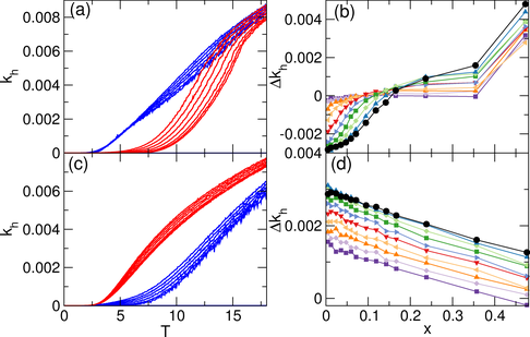
Figure 5: (a) Hopping rate kh vs T for the square ice system. Blue curves: khc for vertices adjacent to doubly-occupied traps; red curves: khf for vertices not adjacent to doubly-occupied traps. The curves are plotted for x = 0, 0.00945, 0.0236, 0.0472, 0.0709, 0.0945, and 0.1181, from the bottom red (blue) curve to the top red (blue) curve. The hopping rate is enhanced near the doping sites in the square ice. (b) The difference in the hopping rates ∆kh=khfkhc vs x for T=8 (black circles), T=9 (dark blue up triangles), T=10 (light green diamonds), T=11 (dark green squares), T=12 (light blue right triangles), T=13 (red down triangles), T=14 (light orange left triangles), T=15 (dark orange up triangles), T=16 (light purple diamonds), and T=17 (dark purple squares). For small values of x, ∆kh is negative since the hopping rate is highest close to the doping sites, and it approaches zero as the doping level or temperature is increased. (c) khc (blue) and khf (red) vs T for the kagome ice at x = 0, 0.0094, 0.0238, 0.0476, 0.07142, 0.0952, and 0.119 from the bottom red (blue) curve to the top red (blue) curve. Here the trend in the hopping rate is reversed, with the lowest hopping rates close to the doping sites. (d) δkh vs x for the kagome ice for T=8 to 17 from top to bottom, with the same symbols as in panel (b).
Fig6.png
Figure 6: The spatial distribution of the thermally induced hopping in the entire sample at T = 12.0. Black circles indicate the doped traps. Hopping rates are indicated on a color scale where red sites have high kh and blue sites have low kh. (a) In the kagome ice at x = 0.07142, traps near the doping sites have suppressed hopping rates. (b) In the square ice system at x = 0.0709, traps near the doping sites have increased hopping rates.

5.  Dynamics

To further quantify the different effects of doping in the square and kagome ices, we examine the hopping rate kh at which the colloids jump from one well to the other inside the double-well traps, in units of inverse simulation time steps. We average kh over two colloid populations: khc is the average hopping rate for all colloids in traps that are next to doped, doubly-occupied traps, while khf is the average hopping rate for the colloids in traps that are not next to doping sites. Here, a trap is defined to be next to a doping site if it is part of a vertex that includes the doped trap. In Fig. 5(a) we plot khc and khf versus T for square ice samples with x ranging from x=0 to x=0.1181. For finite doping, khc for the traps close to doping sites increases from zero near T=2, while khf for the traps that are away from doping sites does not begin to increase until T=5 to 7. The temperature at which the initial upturn of khf occurs decreases with increasing x, caused when the hopping barrier in an undoped site is depressed by proximity to two or more doped sites, an arrangement that becomes more common as x increases. This effect appears more clearly in Fig. 6(b) where we plot the spatial distribution of hopping rates in a square ice system with x = 0.0709 at T = 12. Here the largest hopping rates occur for traps that are immediately adjacent to two or more doping sites. In Fig. 5(b) we plot the difference in the hopping rates ∆kh=khfkhc as a function of x for square ice samples with T = 8 to 17. For low doping x < 0.2, the magnitude of ∆kh is largest at low temperatures and gradually diminishes to zero as the temperature increases. For x > 0.2 we find a reversal in the relative hopping rates, where the hopping switches from being more rapid close to doping sites at low x to being more rapid away from doping sites at higher x. This reflects a transition to a regime where the density of doped sites becomes high enough to strongly constrain the colloid positions in many undoped sites due to random clustering of the doped sites, so that traps close to doped sites have a suppressed rate of thermally induced hopping.
In Fig. 5(c) we plot the hopping rates khc and khf versus T for the kagome ice at doping levels x = 0.0095 to 0.119. Here we find the opposite behavior from the square ice, with colloids in traps next to doping sites having a significantly lower hopping rate than colloids in traps that are away from doping sites. Figure 5(d) shows ∆kh is largest at the lowest temperatures and monotonically decreases both with increasing T and with increasing x. In Fig. 6(a) we illustrate the spatial distribution of the hopping rates in the kagome ice for x=0.0714 at T = 12, where the lowest hopping rates appear adjacent to the doped sites. The clustering effect observed for the hopping rate in the square ice system, where there is a change in sign of ∆kh as the doping level increases, is absent in the kagome ice. These results show that doping has opposite effects on square and kagome ices. Since the square ice has an ordered ground state, the doping adds local frustration which serves as weak spots at which hopping can more readily occur. In the kagome ice, the ground state is not ordered, and doping instead lifts the local degeneracy to create "hard" spots at which the hopping rate is suppressed.

6.  Summary

In summary, we have examined the effect of doping on square and kagome artificial spin ice systems constructed from colloids in double well traps. Doping is introduced by adding an extra colloid to a single trap to create an effective spin that is pointing both in and out of the corresponding vertex. For the square ice, doping creates additional monopole excitations that serve to screen the doped site from the bulk. As the temperature increases, these screening monopoles begin to move away from the doping sites by generating additional monopoles or a string of biased ground state vertices. The doping sites create local weak spots at which local thermal disordering can readily occur as the temperature is increased. For kagome ice, we find the opposite effect, with no additional monopoles created by doping since a shift in the population of ground state vertices serves to absorb the extra charge introduced by doping, while there is a reduction of the hopping rate of colloids in traps adjacent to the doped sites. The doping can cause a small increase in the fraction of vertices in the ground state configuration at finite temperatures in the kagome ice due to the suppression of the hopping, while for the square ice the doping always decreases the fraction of vertices in the ground state.

  Acknowledgements

We thank C. Nisoli for useful discussions. This work was carried out under the auspices of the NNSA of the U.S. DoE at LANL under Contract No. DE-AC52-06NA25396. The work of AL was supported by a grant of the Romanian National Authority for Scientific Research, CNCS-UEFISCDI, project number PN-II-RU-TE-2011-3-0114.

References

[1]
Wang R F, Nisoli C, Freitas R S, Li J, McConville W, Cooley B J, Lund M S, Samarth N, Leighton C, Crespi V H and Schiffer P 2006 Nature (London) 439 303
[2]
Möller G and Moessner R 2006 Phys. Rev. Lett. 96 237202
[3]
Qi Y, Brintlinger T and Cumings J 2008 Phys. Rev. B 77 094418
[4]
Ladak S, Read D E, Perkins G K, Cohen L F and Branford W R Branford 2010 Nature Phys. 6 359
[5]
Mengotti E, Heyderman L J, Rodríguez A F, Nolting F, Hügli R V and Braun H-B 2011 Nature Phys. 7 67
[6]
Morgan J P, Stein A, Langridge S and Marrows C H 2011 Nature Phys. 7 75
[7]
Branford W R, Ladak S, Read D E, Zeissler K and Cohen L F 2012 Science 335 1597
[8]
Nisoli C, Moessner R and Schiffer P 2013 Rev. Mod. Phys. 85 1473
[9]
Libál A, Reichhardt C J O and Reichhardt C 2009 Phys. Rev. Lett. 102 237004
[10]
Latimer M L, Berdiyorov G R, Xiao Z L, Peeters F M and Kwok W K 2013 Phys. Rev. Lett. 111 067001
[11]
Trastoy J, Malnou M, Ulysse C, Bernard R, Bergeal N, Faini G, Lesueur J, Briatico J and Villegas J E 2014 Nature Nanotech. 9 710
[12]
Libál A, Reichhardt C and Reichhardt C J O 2006 Phys. Rev. Lett. 97 228302
[13]
Han Y, Shokef Y, Alsayed A M, Yunker P, Lubensky T C and Yodh A G 2008 Nature 456 898
[14]
Reichhardt C J O, Libál A and Reichhardt C 2012 New J. Phys. 14 025006
[15]
Mellado P, Concha A and Mahadevan L 2012 Phys. Rev. Lett. 109 257203
[16]
Shokef Y, Han Y, Souslov A, Yodh A G and Lubensky T C 2013 Soft Matter 9 6565
[17]
Chern G-W, Reichhardt C and Reichhardt C J O 2013 Phys. Rev. E 87 062305
[18]
Mellado P, Petrova O, Shen Y and Tchernyshyov O 2010 Phys. Rev. Lett. 105 187206
[19]
Chern G-W, Reichhardt C and Reichhardt C J O 2014 New J. Phys. 16 063051
[20]
Libál A, Reichhardt C and Reichhardt C J O 2012 Phys. Rev. E 86 021406
[21]
Kapaklis V, Arnalds U B, Harman-Clarke A, Papaioannou E T, Karimipour M, Korelis P, Taroni A, Holdsworth P C W, Bramwell S T and Hjorvarsson B 2012 New J. Phys. 14 035009
[22]
Porro J M, Bedoya-Pinto A, Berger A and Vavassori P 2013 New J. Phys. 15 055012
[23]
Levis D, Cugliandolo L F, Foini L and Tarzia M 2013 Phys. Rev. Lett. 110 207206
[24]
Farhan A, Derlet P M, Kleibert A, Balan A, Chopdekar R V, Wyss M, Perron J, Scholl A, Nolting F and Heyderman L J 2013 Nature Phys. 9 375
[25]
Montaigne F, Lacour D, Chioar I A, Rougemaille N, Louis D, Mc Murtry S, Riahi H, Burgos B S, Mentes T O, Locatelli A, Canals B and Hehn M 2014 Sci. Rep 4 5702
[26]
Kapaklis V, Arnalds U B, Farhan A, Chopdekar R V, Balan A, Scholl A, Heyderman L J and Hjorvarsson B Nature Nanotechnol. 9 514
[27]
Pauling L C 1935 J. Am. Chem. Soc. 57 2680
[28]
Anderson P W 1956 Phys. Rev. 102 1008
[29]
Harris M J, Bramwell S T, McMorrow D F, Zeiske T and Godfrey K W 1997 Phys. Rev. Lett. 79 2554
[30]
Ramirez A P, Hayashi A, Cava R J and Siddharthan R 1999 Nature 399 333
[31]
Bramwell S T and Gingras M J P 2001 Science 294 1495
[32]
Mól L A S, Pereira A R and Moura-Melo W A 2012 Phys. Rev. B 85 184410
[33]
Chern G-W, Morrison M J and Nisoli C 2013 Phys. Rev. Lett. 111 177201
[34]
Gilbert I, Chern G-W, Zhang S, O'Brien L, Fore B, Nisoli C and Schiffer P 2014 Nature Phys. 10 670
[35]
Budrikis Z, Morgan J P, Akerman J, Stein A, Politi P, Langridge S, Marrows C H and Stamps R L 2012 Phys. Rev. Lett. 109 037203
[36]
Budrikis Z, Politi P and Stamps R L 2012 New J. Phys. 14 045008
[37]
Silva R, Lopes R, Mól L, Moura-Melo W, Wysin G and Pereira A 2013 Phys. Rev. B 87 014414
[38]
Tajima Y, Matsuo T and Suga H 1982 Nature (London) 299 810
[39]
Barkema G T and de Boer J 1993 J. Chem. Phys. 99 2059
[40]
Salzmann C G, Radaelli P G, Hallbrucker A, Mayer E and Finney J L 2006 Science 311 1758
[41]
Lau G C, Freitas R S, Ueland B G, Muegge B D, Duncan E L, Schiffer P and Cava R J Nature Phys. 2 249
[42]
Sen A and Moessner R arXiv:1405.0668
[43]
Mangold K, Leiderer P and Bechinger C 2003 Phys. Rev. Lett. 90 158302
[44]
Mikhel J, Roth J, Helden L and Bechinger C 2008 Nature (London) 454 501


File translated from TEX by TTHgold, version 4.00.
Back to Home