Physical Review E 87, 062305 (2013)

Frustrated colloidal ordering and fully packed loops in arrays of optical traps

Gia-Wei Chern, C. Reichhardt, and C. J. Olson Reichhardt

Center for Nonlinear Studies and Theoretical Division, Los Alamos National Laboratory, Los Alamos, New Mexico 87545, USA

(Received 12 February 2013; published 10 June 2013)

We propose that a system of colloidal particles interacting with a honeycomb array of optical traps that each contain three wells can be used to realize a fully packed loop model. One of the phases in this system can be mapped to Baxter's three-coloring problem, offering an easily accessible physical realization of this problem. As a function of temperature and interaction strength, we find a series of phases, including long range ordered loop or stripe states, stripes with sliding symmetries, random packed loop states, and disordered states in which the loops break apart. Our geometry could be constructed using ion trap arrays, BEC vortices in optical traps, or magnetic vortices in nanostructured superconductors.
I. INTRODUCTION
II. MODEL
References


I.  INTRODUCTION

There has recently been tremendous growth in the area of creating idealized systems in which certain types of statistical mechanics models with and without geometric frustration can be physically realized, such as in nanomagnets [1,2,3] and soft matter systems [4,5,6,7,8,9,10,11,12,13,14]. The key advantage of these systems is that they allow direct experimental access to the microscopic degrees of freedom. One of the most active of these areas has been artificial spin ices created using nanomagnetic arrays with square [1] or hexagonal ordering [2,3], where ordered or frustrated states can occur that mimic real spin ice systems [15]. Here, various types of excitations such as monopoles can arise, and the dynamics can be studied under an external field [3]. There are many other statistical mechanics models that exhibit frustration effects, including loop models such as the famous Baxter's three-coloring model [16], where only very limited work has been performed on proposed physical realizations, all of which involve atomic degrees of freedom [17,18,19,20]. The nanomagnetic systems have certain constraints, such as relatively high levels of disorder and the lack of temperature-like fluctuations, that make it very difficult to realize many other types of statistical mechanics models of interest.
Fig1.png
Figure 1: (a) Schematic diagram of the basic unit cell with two triple well traps each containing one colloidal particle. (b) and (c) are snapshots of a small portion of the system. The green triangles represent the traps and the red dots denote the particles. (b) shows a random distribution of particles at high temperatures. U0 pairs are circled and U1 pairs are boxed. (c) shows an example of a particle configuration that can be mapped to random fully packed loops in the hexagonal lattice, as illustrated in panel (d). The yellow contour in (d) corresponds to a flippable type-II loop.
Here we propose that a system of colloidal particles interacting with optical trap arrays can be used to realize fully packed loop models, and show that one of the resulting phases can be mapped to the three-coloring model. Loop models have been applied to a wide variety of physical systems, ranging from polymer physics [21,22] and turbulence [23] to optics [24] and magnetism [25,26,27], and a physical realization of an idealized loop model would be a major step in this field. Using a colloidal system provides direct experimental access to the microscopic degrees of freedom of such models; in addition, the realization of a three-color model that we describe can not be achieved in magnetic systems due to their intrinsic time-reversal symmetry. Colloidal systems interacting with periodic optical arrays have been experimentally realized [4,5,8,9,10,28] and shown to exhibit novel types of orderings depending on the nature of the substrate [4,8,9,13]. Beyond these static states, it is also possible to study a variety of dynamical processes such as the motion of kinks and antikinks [10,12]. Highly tailored optical trap arrays can be created where the colloidal particles can sit in multiple positions in a single trapping site [5,29,28], so that arrays where colloidal particles can occupy one of three possible positions in a trap are well within current experimental capabilities.


II.  MODEL

We consider a 2D array of N triangular-shaped traps that each contain three potential minima, as illustrated in Fig. 1(a). These traps are similar to those created experimentally in Ref. [4]. The traps form a honeycomb lattice with triangles of opposite orientations occupying the two different sublattices, as shown in Fig. 1(b) and (c). When each trap contains one colloidal particle, the system provides a natural realization of the 3-state Potts model on the honeycomb lattice. We introduce a Potts variable σi = 1, 2, or 3 to denote the potential well occupied by the particle in the i-th trap. In order to characterize the colloidal ordering, we also introduce three unit vectors for each Potts state: e1 = (0, 1), and e2, 3 = (±√3/2, −1/2). The particle in the i-th trap is located at ri = Ri + dσi, where Ri is the center of the trap and the displacement dσ = ±δ eσ, with the plus (minus) sign for up (down) triangles. δ denotes the linear size of the trap.
The colloidal particles interact with each other via a repulsive screened Coulomb or Yukawa potential given by V(rij) = V0 q2 exp(−κrij)/rij. Here rij is the distance between two particles, V0 = Z*2/(4πϵϵ0), Z* is the unit of charge, ϵ is the solvent dielectric constant, q is the dimensionless colloid charge, and 1/κ is the screening length. The Hamiltonian of the model system reads
H = 1

2


i,j 
V(|Rij + dσidσj |)
(1)
where the summation runs over all pairs of triangular traps i, j. Since the particles are always confined to one of the three potential wells in each trap, we can identify the first few neighboring interaction terms of the colloidal potential V(rij) as summarized in Fig. 2. The dominant U0 interaction is between two particles at the closest corners of two neighboring triangles shown in Fig. 2(a). Since these two potential wells are specified by the same Potts state in the respective traps, the U0 term essentially introduces an anisotropic antiferromagnetic interaction between the Potts variables:
H0 = U0

ij 
δαij, σi  δαij, σj,
(2)
where 〈ij 〉 denotes two nearest-neighbor traps, and αij = 1, 2, 3 specifies the relevant Potts state of the adjacent wells of the 〈ij 〉 pair. Such U0-pairs of particles [circled in Fig. 1(b)] are energetically unfavorable and will be suppressed at temperatures T << U0. It is worth noting that the interactions in Eq. (2) are frustrated and there exist extensively degenerate Potts states (colloidal configurations without U0-pairs) that minimize H0.
By attaching an arrow to each particle pointing from the center of the triangular trap to the corner occupied by the particle, the colloidal configuration can be mapped to a collection of directed strings. Since the triangles form a honeycomb lattice, a similar mapping can be established by extending the arrow onto the corresponding bond [see Fig. 1(c) and (d)]. As each trap contains exactly one particle, there is always an outgoing arrow for each vertex of the honeycomb lattice; however, the number of incoming arrows for individual vertices can be 0, 1, or 2. The number of vertices with no incoming arrow must equal the number of vertices with 2 incoming arrows since these are the sources and sinks (or end points) of the directed strings. The second and most relevant U1 term of the interaction, shown in Fig. 2(b), prevents the fusion of two strings by penalizing vertices with two incoming arrows. Examples of U1 pairs are highlighted by square boxes in Fig. 1(b). The number of end point vertices is suppressed at temperatures T << U1, where for systems with periodic boundary conditions (BC) it becomes energetically more favorable for strings to form closed loops as shown in Figs. 1(c) and (d) [30,31]. For finite lattices with open BC, the end points of the strings reside at the boundaries of the system. The further-neighbor interactions U2 and U3 shown in Fig. 2(c,d) induce long-range ordering of particles at very low temperatures. In particular, the U2b term favors alignment of particles in two different alternating Potts states along one of the C3 symmetry directions, effectively introducing a bending stiffness to the strings.
Fig2.png
Figure 2: Various interaction terms arising from the screened-Coulomb or Yukawa potential V(rij) between a pair of colloids in the optical traps.
It is worth noting that each fully packed loop (FPL) configuration on the honeycomb can be further mapped to a three-colored configuration on the same lattice. In Baxter's three coloring model [16], each bond of the honeycomb lattice is assigned a color R, G, or B, so that three different colors meet at each vertex, and all such configurations are given equal statistical weight. The R and B colored bonds thus form a FPL configuration as illustrated in Fig. 1(d), and the two different sequences RBRB… and BRBR… correspond to the forward and backward propagating loops, respectively. It is important to note that all three-colored configurations are energetically degenerate if we retain interactions up to the U1 terms only. Long-range orderings are induced by the further-distance interactions in V(rij).
To understand the various phases of the model system, we perform Monte Carlo simulations on the effective 3-state Potts model described by Eq. (1). Our choice of algorithm varies depending on the temperature. At high temperatures, the standard single-site Metropolis updates are sufficient to equilibrate the system; however, such local updates experience a dynamical freezing at temperatures T << U1 due to the huge energy cost of updating a single-site Potts state. Since the effective degrees of freedom in this temperature regime are the fully packed loops discussed above, we also implement two types of non-local updates in our Monte Carlo simulations similar to the loop algorithm introduced for the three-coloring problem [32]. In the first type of loop update, we randomly select a loop of head-to-tail arrows, or a RBRB … loop, and flip all the arrows; this move is accepted according to the standard Metropolis conditions with further-distance interactions U2, U3, … taken into account. The type-II loops consist of alternating bonds with and without arrows; they correspond to the GB or GR-colored loops in the 3-color scheme. An example type-II loop is shown in Fig. 1(d).
At very low temperatures, even the loop updates suffer freezing problems. Unlike the loops in dimer or spin-ice models [33,34], which can be constructed step by step from numerous possible paths, the loops in the three-coloring problem are predetermined by the colors in a given configuration. The so-called worm algorithm [35], in which detailed balance is always satisfied when constructing the loop, cannot be applied to our case. The freezing problem arises because the acceptance rate of flipping a long loop in the standard Metropolis criterion becomes exceedingly small at low T. To overcome this problem, we employ the parallel tempering algorithm [36] to simulate this low-temperature regime. By simultaneously simulating 150 replicas covering a temperature window 0 < T < 0.1 U1, we are able to fully equilibrate a system with periodic boundary conditions containing N = 2×6×12 particles; the results from a system with linear trap size δ = 0.9×(a/2√3) and screening length κ−1=0.06 a, where a is the lattice constant of the underlying honeycomb lattice, are summarized in Fig. 3.
Fig3.png
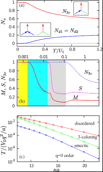
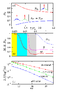
Figure 3: (a) Nv, the fraction of vertices of type v, as a function of temperature T/U1. Upper red line: N3c; lower blue line: Nd1+Nd2; dashed line: all other vertex types. Insets: schematics of the three low-temperature vertex types Nd1, Nd2, and N3c. 
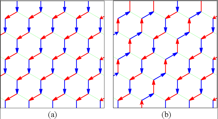
(b) Order parameters M and S along with N3c as a function of temperature T/U1. The parameter M characterizes a uniform long-range ordering of particles in which all loops are directed in the same direction and parallel to each other. The stripe order parameter S describes a partially ordered phase in which loops are parallel to each other but the direction of individual loops is disordered. (c) Phase diagram of temperature T in units of V0q2/a vs κa showing the regions in which the ordered, smectic, three-coloring, and disordered states are observed. Red circles: T3c; green squares: TS; blue triangles: TN.
In Fig. 3(a) we plot the fraction Nv of honeycomb lattice vertices of type v as a function of temperature in the regime T << U0. Since the occurrence of U0-pairs is strongly suppressed in this regime, there exist only three vertex types Nd1, Nd2, and N3c, defined according to the `coloring' of the three bonds attached to the vertex, as illustrated in the insets of Fig. 3(a). The three bonds meeting at the lowest-energy N3c vertices always have different colors. In the language of loops, these 3-color vertices have exactly one incoming and one outgoing arrow. There are two types, Nd1 and Nd2, of higher-energy defect vertices that violate the three-color constraints; they correspond to the sources and sinks of the open strings, and always satisfy Nd1=Nd2. In Fig. 3(a), as T decreases the fraction of defect vertices Nd1+Nd2 gradually decreases before vanishing for T < T3c ≈ 0.1 U1, while the fraction of 3-color vertices N3c saturates to 1 at low T. We define the crossover temperature T3c as the point at which the fraction of defect vertices drops below 0.1%. Below T3c, the system can be mapped to a three-colored or fully-packed loops configuration. The particle-particle correlations in this disordered yet highly constrained phase are expected to exhibit a quasi-power-law decay [16]. We find that g(r) for our system in the 3-coloring regime approaches n = 1/3 for large separations, as shown in Fig. 4. The density-density correlation function Cnn(r)=〈n1(r)n1(0)〉−n2 along one of the C3 axes follows a power law decay at large r with an exponent of 4/3, as expected for a three-colored configuration and as illustrated in the inset of Fig. 4. Here n1(r) is the density of particles at a particular potential well, such as well number 1, of an up triangular trap.
As discussed previously, the further-neighbor interactions U2 and U3 induce long-range orderings of loops at lower temperatures. In particular, the loops acquire a bending stiffness due to the U2b interaction. As a result, the loops start to align themselves with one of the three principle lattice symmetry directions upon lowering the temperature. Since the dominant Potts interaction U0 is antiferromagnetic, we consider a Néel type order parameter: M = (2/√3N) ∑i (−1)i eσi, where (−1)i = +1 for up triangles and −1 for down triangles. The order parameter M = |M| indeed rises to its maximum at T <~TN ≈ 0.003 U1 as shown in Fig. 3(b), indicating a ground state with long-range antiferro-Potts order. The phase boundary TN shown in Fig. 3(c) is defined as the point at which M reaches 99% of its maximum value. One of the perfectly ordered states is illustrated in Fig. 5(a); there are a total of 6 degenerate ground states related to the breaking of Z2 sublattice (the arrows in the loops) and C3 rotational (the orientation of the loops) symmetries.
Fig4.png
Figure 4: Particle pair distribution function g(r) in the 3-coloring regime (T = 0.08 U1 with κ−1 = 0.06 a) obtained from Monte Carlo simulations with loop algorithms on a system with 2×1202 particles. At large separation g(r) → n = 1/3. The inset shows the density-density correlation function Cnn(r) = 〈n1(r) n1(0) 〉− n2 along one of the C3 axes. The correlation exhibits a power-law r−4/3 decay at large r.
Interestingly, for decreasing temperature the order parameter M shows an upturn at TS ≈ 0.034 U1, above the onset of long-range Potts order. Examination of the snapshots from Monte Carlo simulations shows a partially ordered phase with additional sliding symmetries [37]. In this phase, the loops are either parallel or antiparallel to each other, hence breaking the C3 lattice rotational symmetry. The directions of arrows in individual loops remain disordered as shown in Fig. 5(b). This partially ordered phase is characterized by a Z3 order parameter indicating the overall orientation of loops and a set of Ising variables { τ0, τ1, …, τL} specifying the direction of each loop. To characterize this stripe-like order, we first compute the antiferro-Potts order on a 1D chain along one of the C3 axes: mα(c) = (1/L) vα·∑nc (−1)n eσn, where n is a site index along the chain c; α = 1, 2, 3 specifying the orientation of the chains; and vα = eβeγ, where (αβγ) is a cyclic permutation of (123). The vector vα is used to project the vector sum to the relevant Potts states along the chain. Averaging over chains of the same orientation α gives a quasi-1D order parameter: Mα = (1/L) ∑c |mα(c)|, and finally the stripe order parameter is defined as their maximum S = maxα Mα. As shown in Fig. 3(b), the system enters the partially ordered stripe phase at T <~TS as the order parameter S saturates to its maximum. The phase boundary TS shown in Fig. 3(c) is determined by the crossing point of Binder's cumulants from 6×6, 6×9, 9×9, and 6×12 lattices.
We summarize the sequence of thermodynamic transformations, illustrated in the phase diagram in Fig. 3(c), as follows. As the temperature is lowered, the colloidal system first undergoes a crossover into the 3-color or random FPL phase at T3c  ∼ O(U1) . A phase transition into the partially ordered phase occurs at TS  ∼ O(U2b) when the stripe-ordering arises from the positive bending energy produced by the U2b interaction. Finally, the system undergoes another phase transition into the long-range antiferro-Potts ordered ground state at TN. We note that for larger system sizes, our Monte Carlo simulations combining local Metropolis, loop updates, and parallel tempering are able to reach the equilibrium 3-color phase at T < T3c. However, since full equilibration to the partially ordered striped phase as well as the fully ordered ground state requires flipping system-size loops, which costs too much energy for larger lattices, our algorithm can only produce a multi-domain stripe phase. It is worth noting that in the thermodynamic limit, the system cannot reach the true long-range order and stays in this smectic-like phase due to the huge energy barrier separating different stripe states. Our smectic phase is distinct from a q=0 phase with domains. Conventionally, domain walls are topological defects that separate domains of (usually exact) degenerate ground states of the Hamiltonian, where the degeneracy usually arises from the symmetry of the Hamiltonian. In our case, however, the different layered states are almost degenerate mainly due to frustration and are accidental, meaning that they are not protected by symmetry. The system is unable to reach the true q=0 ground state due to dynamical freezing at low T from the large energy barriers separating the layered states.
Fig5.png
Figure 5: (a) A long-range ordered loop state characterized by an antiferromagnetic Potts order parameter M. The parallel loops in this ordered state are directed in the same direction. (b) A partially ordered loop state exhibiting a sliding symmetry. The loops in this phase are parallel to each other but the direction of individual loops remains disordered. This state is characterized by the stripe order parameter S.
It is interesting to note that the highly degenerate kagome-ice manifold [38,39] can be derived from the 3-coloring manifold by re-coloring every G bond to B color; the number of B bonds is thus twice the number of R bonds in the mapped configuration. By identifying the R bonds as the minority spins, e.g. the out-spin in a two-in-one-out triangle, the re-colored 3-coloring state is mapped to a spin configuration in kagome ice. This mapping can be physically realized in our colloidal system by increasing the particle numbers such that all 3c vertices are replaced by d1 defect vertices [see inset of Fig. 3(a)]. Although correlation functions in both phases are critical, the kagome-ice phase is described by a scalar Gaussian field, while the effective field theory for the 3-coloring model requires a two-component vector field [40].
In summary, we have proposed that colloidal particles interacting with a honeycomb array of optical traps that each contain three wells can be used to realize a fully packed loop model. We show that this system exhibits an ordered ground state, a smectic-like stripe phase with a sliding symmetry, a random fully packed loop state, and a disordered state with broken loops. The random fully packed loop state can be mapped to Baxter's three-coloring problem, indicating that our system could be used to create a physical realization of this problem. We map out where these phases occur as a function of temperature and interaction strength. Fully packed loops on different lattices can be similarly realized with optical arrays in which the number of potential wells in a trap site is the same as its coordination number. Our results should be generalizible to other systems of repulsively interacting particles in a similar array of three-well traps, such as for vortices in BEC's interacting with optical arrays, vortices in nanostructured type-II superconductors, and ions in tailored trap arrays.
This work was carried out under the auspices of the NNSA of the U.S. DoE at LANL under Contract No. DE-AC52-06NA25396.

References

[1]
R. F. Wang et al, Nature (London) 439, 303 (2006); J. P. Morgan, A. Stein, S. Langridge, and C. H. Marrows, Nature Phys. 7, 75 (2011); Z. Budrikis, J.P. Morgan, J. Akerman, A. Stein, P. Politi, S. Langridge, C.H. Marrows, and R.L. Stamps, Phys. Rev. Lett. 109, 037203 (2012).
[2]
Y. Qi, T. Brintlinger and J. Cumings, Phys. Rev. B 77, 094418 (2008); P.E. Lammert, X. Ke, J. Li, C. Nisoli, D.M. Garand, V.H. Crespi, and P. Schiffer, Nature Phys. 6, 786 (2010).
[3]
E. Mengotti, L.J. Heyderman, A.F. Rodriguez, F. Nolting , R.V. Hugli, and H.-B. Braun, Nature Phys. 7, 68 (2011); S. Ladak, D.E. Read, G.K. Perkins, L.F. Cohen, and W.R. Branford, ibid. 6, 359 (2010).
[4]
M. Brunner and C. Bechinger, Phys. Rev. Lett. 88, 248302 (2002).
[5]
D. Babic, C. Schmitt, and C. Bechinger, Chaos 15, 026114 (2005).
[6]
A. Libál, C. Reichhardt, and C. J. Olson Reichhardt, Phys. Rev. Lett. 97, 228302 (2006).
[7]
P. Mellado, A. Concha, and L. Mahadevan, Phys. Rev. Lett. 109, 257203 (2012).
[8]
J. Mikhael, J. Roth, L. Helden, and C. Bechinger, Nature (London) 454, 501 (2008); M. Schmiedeberg, J. Mikhael, S. Rausch, J. Roth, L. Helden, C. Bechinger, and H. Stark, Eur. Phys. J. E 32, 25 (2010).
[9]
P. T. Korda, G. C. Spalding and D. G. Grier, Phys. Rev. B 66, 024504 (2002); K. Mangold, P. Leiderer, and C. Bechinger, Phys. Rev. Lett. 90, 158302 (2003).
[10]
T. Bohlein, J. Mikhael, and C. Bechinger, Nature Mater. 11, 126 (2012).
[11]
Y. Han, Y. Shokef, A.M. Alsayed, P. Yunker, T.C. Lubensky, and A.G. Yodh, Nature (London) 456, 898 (2008).
[12]
A. Vanossi, N. Manni, and E. Tosatti, Proc. Nat. Acad. Sci. (USA) 109, 16429 (2012).
[13]
C. Reichhardt and C.J. Olson, Phys. Rev. Lett. 88, 248301 (2002); R. Agra, F. van Wijland, and E. Trizac, Phys. Rev. Lett. 93, 018304 (2004); A. Sarlah, T. Franosch, and E. Frey, Phys. Rev. Lett. 95, 088302 (2005).
[14]
C. J. Olson Reichhardt, A. Libál, and C. Reichhardt, New J. Phys. 14, 025006 (2012).
[15]
R. Moessner and A.P. Ramirez, Phys. Today 59, 24 (2006).
[16]
R. J.  Baxter, J. Math. Phys. 11, 784 (1970).
[17]
J.E. Moore and D.H. Lee, Phys. Rev. B 69, 104511 (2004).
[18]
C. Castelnovo, P. Pujol, and C. Chamon, Phys. Rev. B 69, 104529 (2004).
[19]
C. Xu and J.E. Moore, Phys. Rev. B 72, 064455 (2005); ibid 76, 104427 (2007).
[20]
Y.-Z. You, Z. Chen, X.-Q. Sun, and H. Zhai, Phys. Rev. Lett. 109, 265302 (2012).
[21]
B. Duplantier, Phys. Rev. Lett. 81, 5489 (1998).
[22]
P. G. de Gennes, Scaling concepts in polymer physics (Cornell Univ. Press, Ithaca, 1979).
[23]
D. Bernard et al., Nature Phys. 2, 124 (2006).
[24]
K. O'Holleran et al., Phys. Rev. Lett. 100, 053902 (2008).
[25]
M. Viret et al., Phys. Rev. Lett. 93, 217402 (2004).
[26]
A. Nahum, J. T. Chalker, P. Serna, M Ortuño, and A. M. Somoza, Phys. Rev. Lett. 107, 110601 (2011).
[27]
L. D. C. Jaubert, M. Haque, and R. Moessner, Phys. Rev. Lett. 107, 177202 (2011).
[28]
K. Dholakia, G. Spalding, and M. MacDonald, Physics World 15, 31 (2002).
[29]
D. Babic and C. Bechinger, Phys. Rev. Lett. 94, 148303 (2005).
[30]
H. W. J. Blöte and B. Nienhuis, Phys. Rev. Lett. 72, 1372 (1994).
[31]
J.  Kondev and C. L. Henley, Phys. Rev. Lett. 73, 2786 (1994).
[32]
D. A. Huse and A.D. Rutenberg, Phys. Rev. B 45, 7536 (1992).
[33]
G. T. Barkema, M. E. J. Newman, Phys. Rev. E 57, 1155 (1998).
[34]
F. Alet, J. L. Jacobsen, G. Misguich, V. Pasquier, F. Mila, and M. Troyer, Phys. Rev. Lett. 94, 235702 (2005).
[35]
N. Prokof'ev and B. Svistunov, Phys. Rev. Lett. 87, 160601 (2001).
[36]
K. Hukushima and K. Nemoto, J. Phys. Soc. Jpn. 65, 1604 (1996).
[37]
Z. Nussinov and E. Fradkin, Phys. Rev. B 71, 195120 (2005).
[38]
M. Udagawa, M. Ogata, and Z. Hiroi, J. Phys. Soc. Jpn. 71, 2365 (2002).
[39]
R. Moessner and S. L. Sondhi, Phys. Rev. B 68, 064411 (2003)
[40]
J. Kondev and C. L. Henley, Nucl. Phys. B 464, 540 (1996).


File translated from TEX by TTHgold, version 4.00.

Back to Home