Physical Review E 86, 021406 (2012)

Hysteresis and Return-Point Memory in Colloidal Artificial Spin Ice Systems

A. Libál¹, C. Reichhardt², and C. J. Olson Reichhardt²

¹Faculty of Mathematics and Computer Science, Babes-Bolyai University, RO-400591 Cluj-Napoca, Romania
²Theoretical Division, Los Alamos National Laboratory, Los Alamos, New Mexico 87545, USA

(Received 17 August 2011; revised manuscript received 22 June 2012; published 27 August 2012)

Using computer simulations, we investigate hysteresis loops and return-point memory for artificial square and kagome spin ice systems by cycling an applied bias force and comparing microscopic effective spin configurations throughout the hysteresis cycle. Return-point memory loss is caused by motion of individual defects in kagome ice or of grain boundaries in square ice. In successive cycles, return-point memory is recovered rapidly in kagome ice. Memory is recovered more gradually in square ice due to the extended nature of the grain boundaries. Increasing the amount of quenched disorder increases the defect density but also enhances the return-point memory since the defects become trapped more easily.

I. INTRODUCTION
II. SIMULATION
III. RESULTS
IV. SUMMARY
References

I. INTRODUCTION

Frustration effects arise in many condensed and soft matter systems, such as when geometric constraints prevent collections of interacting elements such as spins or charged particles from simultaneously minimizing all pairwise interaction energies. One of the best known frustrated systems are the spin ices [1,2], named for their similarity to the frustrated proton ordering in water ice [3]. Spin ices have been realized in both two and three dimensions and exhibit interesting excitations such as effective magnetic monopoles [1,4]. More recently, artificial spin ices were created with arrays of nanomagnets [5,6,7,8,9,10,11,12,13,14], colloidal particles [15,16], and vortices in nanostructured superconductors [17]. In artificial ices, direct visualization of the microscopic effective spin configurations is possible, and system parameters such as interaction strength, doping, or the amount of quenched disorder can be controlled. Under a varying external field, changes in the microscopic configurations can be imaged and used to construct hysteresis loops [9,8,7,14], as shown for kagome ice where the motion, creation, and annihilation of topological defects along the hysteresis cycle were demonstrated [7]. Memory effects are generally associated with hysteresis, and in return-point memory (RPM), the system returns to the same microscopic configuration after completing a hysteresis loop [18,19,20,21,22]. Recently developed techniques show that in real magnetic materials, RPM occurs in strongly disordered samples and is absent for weak disorder when the system becomes too soft to remember its previous state [19,20,22]. Certain classes of T=0 disordered spin systems, such as the random field Ising model [18], exhibit perfect RPM, while other systems require many loops to organize into a state with RPM [21,20]. In more general disordered systems, an RPM-like effect was recently observed in the form of random reorganization into a reversible state for assemblies of interacting particles subjected to a cyclic shear [23]. Insights into magnetic RPM may offer a better understanding of such reversible-irreversible transitions that have been observed in a broad range of systems [24].

Artificial spin ices are an ideal system for studying RPM since they exhibit hysteresis and the microscopic states can be visualized directly. The type of topological defect that forms and its mobility varies in different ice systems, ranging from mobile monopoles [9,7] in kagome ice to less mobile grain boundaries [17,6] in square ice, and this could modify the RPM behavior. To quantify this, we perform numerical simulations of hysteresis in artificial square and kagome spin ices constructed from colloids in double-well traps with varied amounts of quenched disorder. Our model was previously shown to capture the behavior of square and kagome ices [15,17], and the number and type of topological defects present can be controlled by changing the amount of quenched disorder [17]. We use molecular dynamics simulations to capture the motion of extended objects such as grain boundaries. Our work implies that RPM phenomena can be studied in general artificial spin systems where a spin degree of freedom can be defined, as well as in artificial spin ice systems where geometrical frustration of the effective spins is present. This provides a new method for exploring microscopic memory effects in condensed matter systems.

II. SIMULATION

We simulate an artificial spin ice of N charged colloidal particles trapped in an array of elongated double-well pinning sites that have two states determined by which well is occupied by the colloid. The dynamics of colloid i is governed by the overdamped equation of motion η(dR_i/dt)=F_i^cc+F_i^s+F_ext, where the damping constant η = 1. The colloid-colloid interaction force has a Yukawa or screened Coulomb form, F_i^cc = −F₀q²∑^N_{i ≠ j}∇_i V(R_ij), with V(R_ij) = (1/R_ij)exp(−κR_ij)∧r_ij. Here R_ij=|R_i − R_j|, ∧R_ij=(R_i−R_j)/R_ij, R_i(j) is the position of particle i(j), F₀=Z^*2/(4πϵϵ₀), Z^* is the unit of charge, ϵ is the solvent dielectric constant, q is the dimensionless colloid charge, 1/κ = 4a₀ is the screening length, and a₀ is the unit of distance that is typically of order a micron. We neglect hydrodynamic interactions between colloids since we work in the low volume fraction limit and the colloids remain confined in the pins. The pinning force F_s arises from N_p elongated traps of length l=1.333a₀, width d_p=0.4a₀, and depth f_p=100F₀. The pin ends are parabolic confining potentials with radius r_p=0.2a₀. A cylindrical force restricts motion in the direction perpendicular to the long axis of the pinning site, and a barrier in the center of the pinning site is produced by a repulsive parabolic force of height f_r that creates two energy minima on either end of the pin [15]. For square ice the pins are arranged with v=4 traps meeting at each vertex, while for kagome ice, v=3 traps meet at each vertex [17], as shown in Fig. 1. The distance between adjacent vertices is a=2a₀ and there are N_v vertices. Our square ice has 35 ×35 vertices (N_v=1225) and N_p=2450 elongated pins, while our kagome ice has 40 ×40 vertices (N_v=1600) and N_p=2400 elongated pins. Systems of larger size show the same behavior. Disorder is added to the system by increasing or decreasing f_r in individual pinning sites according to a normal distribution with mean f_b=1.0F₀ and standard deviation σ. This is analogous to varied island coercive fields in the nanomagnetic system. We initialize the system by placing a colloid in one randomly selected end of each pinning site so that N=N_p. To construct a hysteresis loop we apply an external force F_ext=F_ext∧n uniformly to the sample, which for charged colloidal particles could be achieved using an external electric field. In the kagome ice ∧n=∧x, while in the square ice ∧n=√2(∧x+∧y)/2, as illustrated in Fig. 1. For large enough F_ext, the sample saturates into a biased ground state determined by the direction of F_ext. The two types of biased ground state vertices are illustrated for both ices in Fig. 1. We sweep F_ext from zero to a positive maximum value F_max at a rate of δF_ext=0.005 every 5000 simulation steps, then back down through zero to a negative maximum value −F_max, and finally back up to zero to create one loop. Our results are unchanged for slower sweep rates using smaller values of δF_ext. The initial curve is defined as the first sweep up of F_ext to F_max after the sample has been prepared in a random state.

Figure 1: (Color online) Schematic of a portion of the artificial ice samples. A charged colloid (dots) can sit in either end of each trap (lozenges). Dark green (light yellow) traps surround vertices that are in a positively (negatively) biased ground state. (a) Square ice, with F_ext applied at θ = 45^° from the x axis. (b) Kagome ice, with F_ext applied along the x axis.

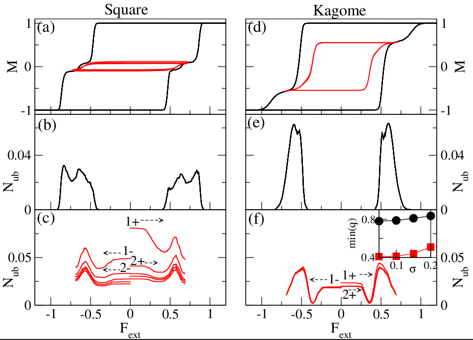
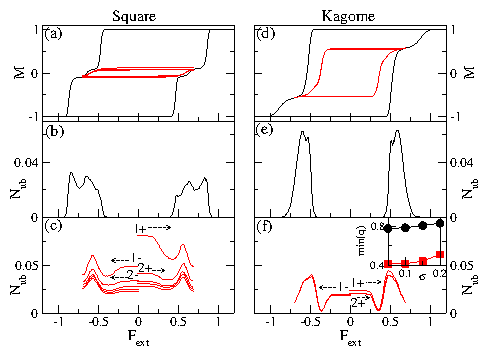
Figure 2: (Color online) (a,b,c) Square ice sample with σ = 0.1. (d,e,f) Kagome ice sample with σ = 0.1. All curves are averaged over ten disorder realizations. (a,d) The reduced magnetization m vs F_ext. Saturation occurs at m = ±1.0 when all the vertices are in biased states. Outer line: Saturated loop with F_max=2.0. Inner lines: Consecutive loops with F_max=0.7, below saturation. The initial curves are not shown. (b,e) Fraction of unbiased vertices N_ub vs F_ext for the saturated loop with F_max=2.0. (c,f) N_ub vs F_ext for repeated unsaturated loops with F_max=0.7, with cycle number n increasing from top to bottom. For clarity, we omit the horizontal lines connecting F_ext=±F_max to F_ext=0. The first few half cycles are labeled; dotted arrows indicate sweep direction for the labeled curves. There is a much greater decrease in N_ub for the square ice than for the kagome ice. 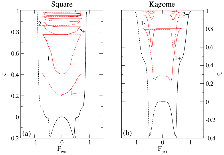Inset of (f): min(q), the effective spin overlap in the n=2 cycle, vs σ for (circles) kagome and (squares) square ice. Samples with stronger disorder have higher q values.

Figure 3: (Color online) (a) Magnetization m vs F_ext and (b) number of defects N_ub vs F_ext for saturated loops with F_max=2.0 obtained for the square ice system in Fig. 2(a-c) using different sweep rates δF_ext. Black filled circles: δF_ext=0.005, the rate used throughout the paper. Red filled symbols indicate slower sweep rates. Filled triangles: δF_ext=0.0005; filled squares: δF_ext=0.0010; filled diamonds: δF_ext=0.0025. Blue open symbols indicate faster sweep rates. Open triangles: δF_ext=0.01; open squares: δF_ext=0.025; open diamonds: δF_ext=0.05. The curves for δF_ext=0.005 are nearly indistinguishable from curves obtained for slower sweep rates, indicating that we are working in the quasistatic regime in the paper. (c) Magnetization m vs F_ext and (d) number of defects N_ub vs F_ext for saturated loops with F_max=2.0 obtained for the square ice system in Fig. 2(a-c) with the same pinning density in samples of different size containing N_v pins. Black filled circles: N_p=3528; red open squares: N_p=4802; green filled diamonds: N_p=6272; blue open triangles: N_p=7938; black plus signs: N_p=9800. The system size considered in Fig. 2(a-c) is already large enough to be in the regime where no significant size dependence of the results appears.

III. RESULTS

We first show that our model captures the hysteretic behavior observed in artificial ice systems [9,8,7,19]. In the absence of quenched disorder or drive, we find ice-rule obeying states that are ordered ground states in the square ice [15] and disordered in the kagome ice. When we add quenched disorder with σ > 0, due to its lack of extensive degeneracy the square ice forms grain boundaries composed of non-ice rule obeying vertices as shown in simulation [17] and experiment [6], while in kagome ice isolated non-ice rule defects appear [17,7]. We define the reduced magnetization m as the projection of the effective spin of each trap onto the driving direction, m=N_v⁻¹∑_i=1^N_ps_i^eff ·∧n, where s_i^eff is a unit vector defined to point from the empty end of the trap to the filled end of the trap. In Fig. 2(a,d) we plot the hysteresis loops for square and kagome ice samples with σ = 0.1. The outer curve is obtained with F_max=2.0, beyond the saturation level where m=±1. We plot the fraction of unbiased vertices N_ub vs F_ext with F_max=2.0 in Fig. 2(b,e). The completely ordered biased states are only destroyed for 0.4 < |F_ext| < 1.0, close to the coercive fields at which the effective spin direction flips. The shape of the hysteresis loop and the peaks in the non-biased defect density in Figs. 2(b,e) are in excellent agreement with the digitally constructed hysteresis loops produced in experiments on nanomagnetic kagome ice samples [9,8,7]. We find the same behavior for slower sweep rates using smaller values of δF_ext and also for larger samples, as shown in Fig. 3. The inner curves in Figs. 2(a,d) show consecutive hysteresis loops obtained below saturation with F_max=0.7, near the middle of the range of F_ext in which the largest number of defects appear. In Fig. 2(c,f) we plot N_ub versus F_ext for the unsaturated hysteresis loops. For the square ice, Fig. 2(c) shows that N_ub decreases with increasing n, where n is the number of loops performed, indicating that defect annihilation is occurring. For continued cycling beyond the number of loops shown in the figure, the system settles into a steady state. In the kagome ice, Fig. 2(f) shows that N_ub hardly changes from one cycle to the next, indicating that only a small number of defects annihilate. For the saturated case with F_max = 2.0 shown in Fig. 2(b,e), the N_ub curves do not evolve under repeated looping since the sample loses all memory of the microscopic configuration near the coercive field once saturation is reached.

Figure 4: (Color online) Effective spin overlap q vs F_ext during consecutive hysteresis loops averaged over ten disorder realizations for (a) a square ice sample with σ = 0.1 and (b) a kagome ice sample with σ = 0.1. Outer line: Saturated loop with F_max=2.0, including the initial curve. Inner lines: Unsaturated loops with F_max=0.7, with n increasing from bottom to top; the first few half loops are labeled. Solid lines: clockwise loops; dashed lines: counterclockwise loops. In the kagome ice, q approaches 1 after only a few cycles, while a much larger number of cycles are required before q approaches 1 in the square ice.

We quantify the RPM by measuring the overlap q in the effective spin configurations along a hysteresis loop [20,22] at equal values of F_ext after n complete cycles. For each trap, we define an effective spin S_i=1 if the colloid is sitting in the right or top end of the trap, and S_i=−1 if the colloid is sitting in the left or bottom end of the trap. Writing the value of S_i after n cycles as S_i⁽ⁿ⁾, we measure

q(F_ext) = N⁻¹

N
∑
i=1

S_i⁽ⁿ⁻¹⁾(F_ext)S_i⁽ⁿ⁾(F_ext) .

(1)

The term in the sum is 1 if the trap was biased in the same direction both before and after the complete cycle, and -1 if the colloid jumped to the other end of the trap. In Fig. 4(a,b) we plot q versus F_ext for both the saturated and unsaturated hysteresis curves in the square and kagome ices shown in Fig. 2(a,d). In the case of the saturated loops, q for the initial curve in Fig. 4(a) shows that since the sample was not initialized in a biased state, the initial configuration differs significantly from the effective spin configuration obtained one cycle later, but for n=2 and above, q=1, indicating perfect memory. For the unsaturated loops obtained with F_max=0.7, q is low during the first cycle, but as n increases q gradually converges to a value just below q=1. A comparison with Fig. 2(c) indicates that the increase in memory with increasing n is correlated with a decrease in N_ub, although for this value of F_max there are always some defected vertices present even after the system reaches a steady state in which the grain boundaries cease to evolve. The kagome ice in Fig. 4(b) shows a similar behavior except that q approaches 1 after only a few cycles, leading to a much faster establishment of RPM than in the square ice. In Fig. 2(f) we show that the number of defected vertices remains nearly constant in the kagome ice even under repeated cycling. This indicates that although the kagome ice defects do not annihilate, they are mobile during the first few cycles and then become pinned. Our results demonstrate that for the square ice, changes in the amount of RPM are primarily associated with the annihilation of defects, while in the kagome ice, RPM is suppressed by the motion of defects.

Although the number of defects N_ub in both types of ice increases with increasing disorder σ, the amount of RPM increases with increasing disorder. We illustrate this in the inset of Fig. 2(f) where we plot the value of q on the n=2 plateau versus σ. A similar effect was observed for real magnetic systems and in spin simulations [19,20,22]. In our system, q increases with increasing disorder due to the stronger pinning of the domain walls in the square ice or of the individual defects in the kagome ice. In the square ice, the disorder prevents the domain walls from coarsening. It was previously shown that as the particle-particle interaction strength in our system is reduced, non-ice-rule obeying vertices begin to appear since their energetic cost decreases [15]. For noninteracting colloids, the sample is strongly disordered but also has perfect RPM since the defected configurations are controlled only by the local disorder and are not modified by particle interactions. Thus we expect that in the experimental nanomagnetic artificial ices, when the coupling is reduced for increased spacing between the nanomagnets, the system should show increased or perfect RPM.

Figure 5: (Color online) Vertices in (a) square ice and (b) kagome ice samples from Fig. 2 during repeated hysteresis cycles. Vertices are colored depending on how many cycles the vertex spends in a defect state, ranging from dark blue for never defected sites to dark red for permanently defected. In (a), motion and annihilation of defects occur near grain boundaries. In (b), individual defects move and are pinned independently without forming grain boundaries.

To illustrate the defect dynamics, in Fig. 5 we plot the vertices colored according to the number of hysteresis cycles each vertex spent as a defected site. Red vertices indicate locations where defects became trapped. Figure 5(a) shows that in the square ice, the defects organize into grain boundaries which move and coarsen under repeated hysteresis cycles. In Fig. 5(b), the kagome ice contains no grain boundaries but has a smaller fraction of intermediately colored vertices compared to the square ice since the isolated defects become trapped after only a few cycles. The square ice grain boundaries are less well pinned than the isolated kagome defects since they are extended objects. These mobile grain boundaries are responsible for the lower amount of RPM found in the square ice compared to the kagome ice. As the grain boundaries become trapped after repeated cycles, RPM increases and eventually saturates. The isolated kagome defects become trapped much more rapidly and their lower density contributes to the overall higher level of RPM in the kagome ice. The motion of individual defects in kagome ice has already been imaged in experiments; it would be interesting to observe whether these defects become localized within a few hysteresis cycles as we predict.

For most artificial ice systems, thermal effects are not relevant; however, thermal fluctuations can be significant in a colloidal system. We find that our results are robust against the addition of weak thermal disorder, and that for T > 0 there is only a slight reduction in the asymptotic value of q and a slight increase in the number of cycles required to reach a steady state. For higher temperatures, RPM is lost even when the system is cycled to saturation since the thermal fluctuations cause random effective spin flips that change the path on each cycle. There is also no increase in RPM under repeated cycles at higher temperature [22].

IV. SUMMARY

In summary, we have studied hysteresis and return-point memory effects for artificial square and kagome ices at the microscopic level. In the square ice for repeated unsaturated hysteresis loop cycles that extend to biases near the coercive field, the RPM increases with each cycle as the grain boundaries present in the sample coarsen and become pinned. In kagome ice the number of defects remains nearly constant under repeated hysteresis cycles and there is much higher RPM. Here, individual defects hop rather than annihilating and are eventually pinned at sites with stronger disorder. The grain boundaries in the square ice are more mobile than the individual defects in the kagome ice since they are extended objects. Our results can be tested readily in different types of artificial ices and also could be studied in more general artificial spin systems.

Acknowledgements

We thank the anonymous referees for their helpful comments. This work was carried out under the auspices of the National Nuclear Security Agency of the U.S. Department of Energy at Los Alamos National Laboratory under Contract No. DE-AC52-06NA25396. A.L. was supported by a grant of the Romanian National Authority for Scientific Research, CNCS - UEFISCDI, project number PN-II-RU-TE-2011-3-0114.

References

[1]: R. Moessner and A.P. Ramirez, Phys. Today 59(2), 24 (2006).
[2]: A.P. Ramirez, A. Hayashi, R.J. Cava, R. Siddharthan, and B.S. Shastry, Nature (London) 399, 333 (1999); S.T. Bramwell and M.J.P. Gingras, Science 294, 1495 (2001).
[3]: L. Pauling, J. Am. Chem. Soc. 57, 2680 (1935).
[4]: C. Castelnovo, R. Moessner, and S.L. Sondhi, Nature (London) 451, 42 (2008); L.D.C. Jaubert and P.C.W. Holdsworth, Nature Phys. 5, 258 (2009); D.J.P. Morris et al., Science 326, 411 (2009); S.T. Bramwell, S.R. Giblin, S. Calder, R. Aldus, D. Prabhakaran, and T. Fennell, Nature (London) 461, 956 (2009).
[5]: R.F. Wang et al., Nature (London) 439, 303 (2006); G. Möller and R. Moessner, Phys. Rev. Lett. 96, 237202 (2006); X. Ke, J. Li, C. Nisoli, P.E. Lammert, W. McConville, R.F. Wang, V.H. Crespi, and P. Schiffer, Phys. Rev. Lett. 101, 037205 (2008); C. Nisoli, J. Li, X. Ke, D. Garand, P. Schiffer, and V.H. Crespi, Phys. Rev. Lett. 105, 047205 (2010); P.E. Lammert, X. Ke, J. Li, C. Nisoli, D.M. Garand, V.H. Crespi, and P. Schiffer, Nature Phys. 6, 786 (2010); J. Li, X. Ke, S. Zhang, D. Garand, C. Nisoli, P. Lammert, V.H. Crespi, and P. Schiffer, Phys. Rev. B 81, 092406 (2010).
[6]: J.P. Morgan, A. Stein, S. Langridge, and C.H. Marrows, Nature Phys. 7, 75 (2011).
[7]: E. Mengotti, L.J. Heyderman, A.F. Rodríguez, F. Nolting, R.V. Hügli, and H.-B. Braun, Nature Phys. 7, 68 (2011).
[8]: A. Schumann, B. Sothmann, P. Szary, and H. Zabel, Appl. Phys. Lett. 97, 022509 (2010).
[9]: O. Tchernyshyov, Nature Phys. 6, 323 (2010); S. Ladak, D.E. Read, G.K. Perkins, L.F. Cohen, and W.R. Branford, ibid. 6, 359 (2010).
[10]: Y. Qi, T. Brintlinger, and J. Cumings, Phys. Rev. B 77, 094418 (2008); E. Mengotti, L.J. Heyderman, A.F. Rodríguez, A. Bisig, L. Le Guyader, F. Nolting, and H.B. Braun, ibid. 78, 144402 (2008); N. Rougemaille et al., Phys. Rev. Lett. 106, 057209 (2011).
[11]: M. Tanaka, E. Saitoh, H. Miyajima, T. Yamaoka, and Y. Iye, Phys. Rev. B 73, 052411 (2006).
[12]: L.A.S. Mol, W.A. Moura-Melo, and A.R. Pereira, Phys. Rev. B 82, 054434 (2010).
[13]: Z. Budrikis, P. Politi, and R.L. Stamps, Phys. Rev. Lett. 105, 017201 (2010); P. Mellado, O. Petrova, Y. Shen, and O. Tchernyshyov, Phys. Rev. Lett. 105, 187206 (2010).
[14]: K.K. Kohli, A.L. Balk, J. Li, S. Zhang, I. Gilbert, P.E. Lammert, V.H. Crespi, P. Schiffer, and N. Samarth, Phys. Rev. B 84, 180412(R) (2011).
[15]: A. Libál, C. Reichhardt, and C.J. Olson Reichhardt, Phys. Rev. Lett. 97, 228302 (2006).
[16]: Y. Han, Y. Shokef, A.M. Alsayed, P. Yunker, T.C. Lubensky, and A.G. Yodh, Nature (London) 456, 898 (2008).
[17]: A. Libál, C.J. Olson Reichhardt, and C. Reichhardt, Phys. Rev. Lett. 102, 237004 (2009); M.L. Latimer, G.R. Berdiyorov, Z.L. Xiao, W.K. Kwok, and F.M. Peeters, Phys. Rev. B 85, 012505 (2012).
[18]: J.P. Sethna, K. Dahmen, S. Kartha, J.A. Krumhansl, B.W. Roberts, and J.D. Shore, Phys. Rev. Lett. 70, 3347 (1993).
[19]: M.S. Pierce et al., Phys. Rev. Lett. 94, 017202 (2005).
[20]: M.S. Pierce et al., Phys. Rev. B 75, 144406 (2007).
[21]: J.M. Deutsch and O. Narayan, Phys. Rev. Lett. 91, 200601 (2003).
[22]: H.G. Katzgraber and G.T Zimanyi, Phys. Rev. B 74, 020405(R) (2006).
[23]: D.J. Pine, J.P. Gollub, J.F. Brady, and A.M. Leshansky, Nature 438, 997 (2005); L. Corte, P.M. Chaikin, J.P. Gollub, and D.J. Pine, Nature Phys. 4, 420 (2008); G.I. Menon and S. Ramaswamy, Phys. Rev. E 79, 061108 (2009).
[24]: N. Mangan, C. Reichhardt, and C.J. Olson Reichhardt, Phys. Rev. Lett. 100, 187002 (2008); C. Reichhardt and C.J. Olson Reichhardt, Phys. Rev. Lett. 103, 168301 (2009); S. Okuma, Y. Tsugawa, and A. Motohashi, Phys. Rev. B 83, 012503 (2011).

File translated from T_EX by T_THgold, version 4.00.

Back to Home