Physical Review Letters 121, 068001 (2018)

Controlled Fluidization, Mobility and Clogging in Obstacle Arrays Using Periodic Perturbations

C. Reichhardt and C.J.O. Reichhardt

Theoretical Division and Center for Nonlinear Studies, Los Alamos National Laboratory, Los Alamos, New Mexico 87545, USA

(Received 25 April 2018; published 7 August 2018)

We show that the clogging susceptibility and flow of particles moving through a random obstacle array can be controlled with a transverse or longitudinal ac drive. The flow rate can vary over several orders of magnitude, and we find both an optimal frequency and an optimal amplitude of driving that maximizes the flow. For dense arrays, at low ac frequencies a heterogeneous creeping clogged phase appears in which rearrangements between different clogged configurations occur. At intermediate frequencies a high mobility fluidized state forms, and at high frequencies the system reenters a heterogeneous frozen clogged state. These results provide a technique for optimizing flow through heterogeneous media that could also serve as the basis for a particle separation method.
Simulation and System
Results
Summary
References

Particle transport through heterogeneous media is relevant to flows in porous media [1,2], transport of colloidal particles on ordered or disordered substrates [3,4,5,6,7], clogging phenomena [8,9,10,11,12,13], filtration [14,15,16], and active matter motion in disordered environments [17,18,19,20]. It also has similarities to systems that exhibit depinning phenomena when driven over random or ordered substrates [21]. Recent work has focused on clogging effects for particle motion through obstacle arrays, where the onset of clogging is characterized by the formation of a heterogeneously dense state [11,12,13]. Such clogging is relevant for the performance of filters or for limiting the amount of flow through disordered media, so understanding how to avoid clog formation or how to optimize the particle mobility in obstacle arrays is highly desirable. Clogging also occurs for particle flow through hoppers or constrictions, where there can be a transition from a flowing to a clogged state as the aperture size decreases [22,23,24,25,26]. The clogging susceptibility in such systems can be reduced with periodic perturbations or vibrations [27,28,29]. Applied perturbations generally produce enhanced flows in disordered systems [30,32,31,33,34]; however, there are examples where the addition of perturbations or noise can decrease the flow or induce jamming, such as the freezing by heating phenomenon [26,35,36] or the appearance of a reentrant high viscosity state in vibrated granular matter [37]. A natural question is whether clogging and mobility for particle flows through obstacles can be controlled or optimized with applied perturbations in the same way as hopper flow. It is also possible to have transverse shaking in hopper like geometries [34] and it would be interesting to understand how transverse and longitudinal ac drives can control the flow in two-dimensional (2D) disordered obstacle arrays, where one type of shaking may be more effective than the other.
In this work we numerically examine particle flow through a disordered obstacle array where the particles experience both a dc drive and ac shaking. In the absence of the ac shaking, this system exhibits a well defined clogging transition at a critical obstacle density ϕcdc as identified in previous work [12] for dc driven disks in obstacle arrays. The clogged states exhibit strong spatial heterogeneity, and ϕcdc remains roughly constant until the disk density approaches the jamming or crystallization density [12]. The previous work focused on the transition to a completely immobile state and the distinction between jamming and clogging behavior. In the present work we measure the disk mobility when a transverse or longitudinal ac drive is added to the system for obstacle densities above ϕcdc, where the ac drive serves to unclog the system. We find that the mobility drops back to zero above a critical obstacle density ϕcac that depends on the frequency and amplitude of the ac drive. We identify an optimal ac frequency and amplitude that optimizes the mobility. low frequencies, the system forms a nearly immobile heterogeneous creeping clogged state, while for intermediate frequencies a more uniform flowing fluidized state appears and at high frequencies a heterogeneous frozen clogged state emerges that resembles the clogged state previously observed for zero ac drive [12]. These results could be applied to control the mobility of particles flowing through random disorder by applying dc and transverse or longitudinal ac drives to systems such as granular matter, colloids, or emulsions. Similar driving protocols could be used for particles with longer range interactions such as superconducting vortices, skyrmions, or charged colloids in disordered media to identify ac driving frequencies that optimize the flow.

Simulation and System

We simulate a 2D system of non-overlapping repulsive particles in the form of disks interacting with a random array of obstacles where the particles are subjected to a dc drift force and an ac shaking force. The sample is of size L ×L with L = 100 and we impose periodic boundary conditions in the x and y directions. Interactions between pairs of disks i and j are given by the repulsive harmonic force Fijdd = k(rij −2Rd)Θ(rij −2Rd)rij, where the disk radius Rd=0.5, rij = |rirj|, rij = (rirj)/rij, and Θ is the Heaviside step function. The spring stiffness k = 200 is large enough that disks overlap by less than one percent, placing us in the hard disk limit as confirmed by previous works [11,12,38]. The obstacles are modeled as immobile disks with the same radius and disk-disk interactions as the mobile particles. There are Nm mobile particles with an area coverage of ϕm = NmπR2d/L2, while the area coverage of the Nobs obstacles is ϕobs = NobsπR2d/L2 and the total area coverage is ϕtot = ϕm + ϕobs. For monodisperse disks the system forms a triangular solid at ϕtot = 0.9 [38]. The obstacles are placed in a dense lattice and randomly diluted until the desired ϕobs is reached, so that the minimum spacing between obstacle centers is dmin=2.0. The particle dynamics are governed by the following overdamped equation of motion: ηd ri/dt = Finteri + Fobsi + Fdc + Fac. Here Finteri=∑j=0NmFddij are the particle-particle interactions, Fobsi=∑k=0NobsFddik are the particle-obstacle interactions, and Fdc = Fdcx is the dc drift force applied in the positive x-direction, where Fdc=0.05. Each simulation time step is of size dt=0.002, and η = 1.0. We apply a sinusoidal ac drive that is either transverse (perpendicular) to the dc drive, Fac=Facy, or longitudinal (parallel) to the dc drive, Fac=Fac||x . We measure the time average of the velocity per particle in the dc drift direction, 〈Vx〉 = Nm−1Nmi = 1vi·x, where vi is the velocity of particle i. We define the mobility as M = 〈Vx〉/ 〈V0x〉, where 〈V0x〉 is the obstacle-free drift velocity, so that in the free flow limit, M = 1.0. After the drive is applied, there is a transient time during which the mobilities settle to a stationary state, so we wait 107 simulation time steps, longer than any of the transient times, before taking measurements. Our results are robust for varied system size, except that in very small samples (L ≤ 20), particles are more likely to become trapped in periodic orbits, giving higher mobilities.
Fig1.png
Figure 1: Locations of particles (red) and obstacles (blue) for a system with ϕtot=0.275 and an x-direction drift force of Fdc = 0.05 under an applied transverse (y-direction) ac drive of magnitude Fac = 0.5 for different ac frequencies ω. (a) A low mobility creeping clogged state with M=0.01 at ω = 10−7 and ϕobs=0.1256. (b) A high mobility fluidized state with M=0.27 at ω = 10−4 and ϕobs=0.1256. (c) A frozen clogged state with M=0 at ω = 10−1 and ϕobs=0.1256. (d) A flowing state at ω = 10−1 and ϕobs = 0.047. The images in (a,b,c) were obtained at the points marked a, b, and c in Fig. 2(b).

Results

In Fig. 1(a) we illustrate the positions of the particles and obstacles in a steady state with Fdc = 0.05, ϕtot=0.275, and ϕobs=0.1256 under a transverse drive of magnitude Fac = 0.5 in what we define as the low frequency limit of ω = 10−7, where the mobility is very small, M=0.01. The particles assemble into high density clogged regions separated by large void areas. There are slow rearrangements of the particles but little net motion in the direction of the dc drift, so the system is effectively transitioning between different clogged configurations. At ω = 10−4 in Fig. 1(b), the mobility of the same sample reaches its maximum value of M = 0.27. Here the clustering is reduced compared to what occurs at lower frequencies, and the system is in a partially fluidized state. For the high frequency of ω = 10−1 in Fig. 1(c), a completely frozen clogged state with M = 0 appears. In Fig. 1(d), when ω = 10−1 but the obstacle density is reduced to ϕobs=0.047, the system is in a flowing state. In the limit of Fac = 0.0 the system in Fig.1(a,b,c) organizes to a completely clogged state while in Fig.1(d) in the same limit the system is flowing.
Fig2.png
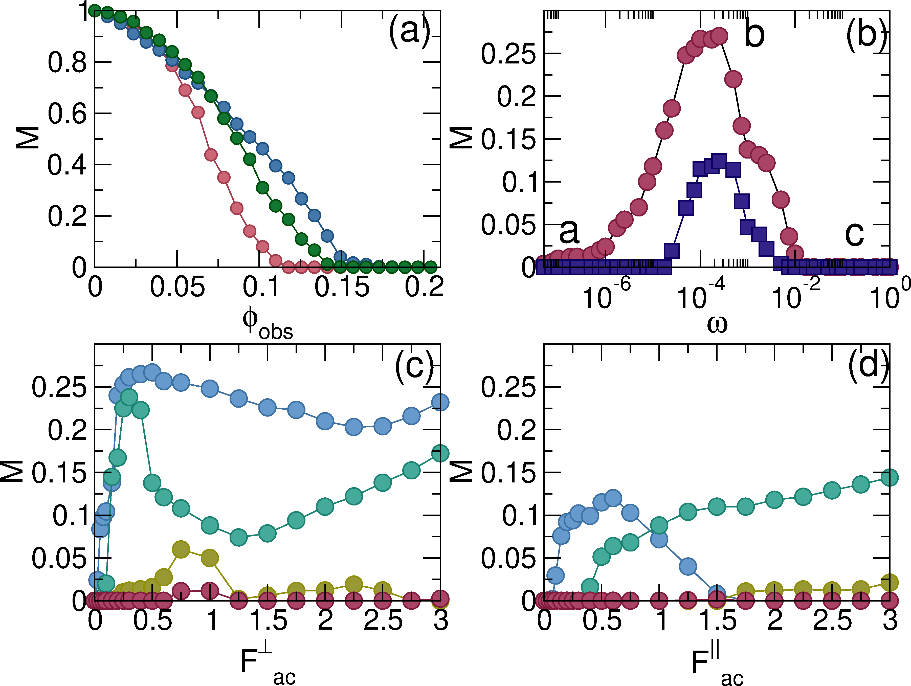
Figure 2: (a) Mobility M vs obstacle density ϕobs for ϕtot = 0.275 at Fac = F||ac=0 (pink), where M = 0 for ϕobs > 0.115; at Fac = 0.5 and ω = 10−4 (blue), where M ≈ 0 for ϕobs > 0.195; and at F||ac = 0.5 and ω = 10−4 (green), where M ≈ 0 for ϕobs > 0.155. 
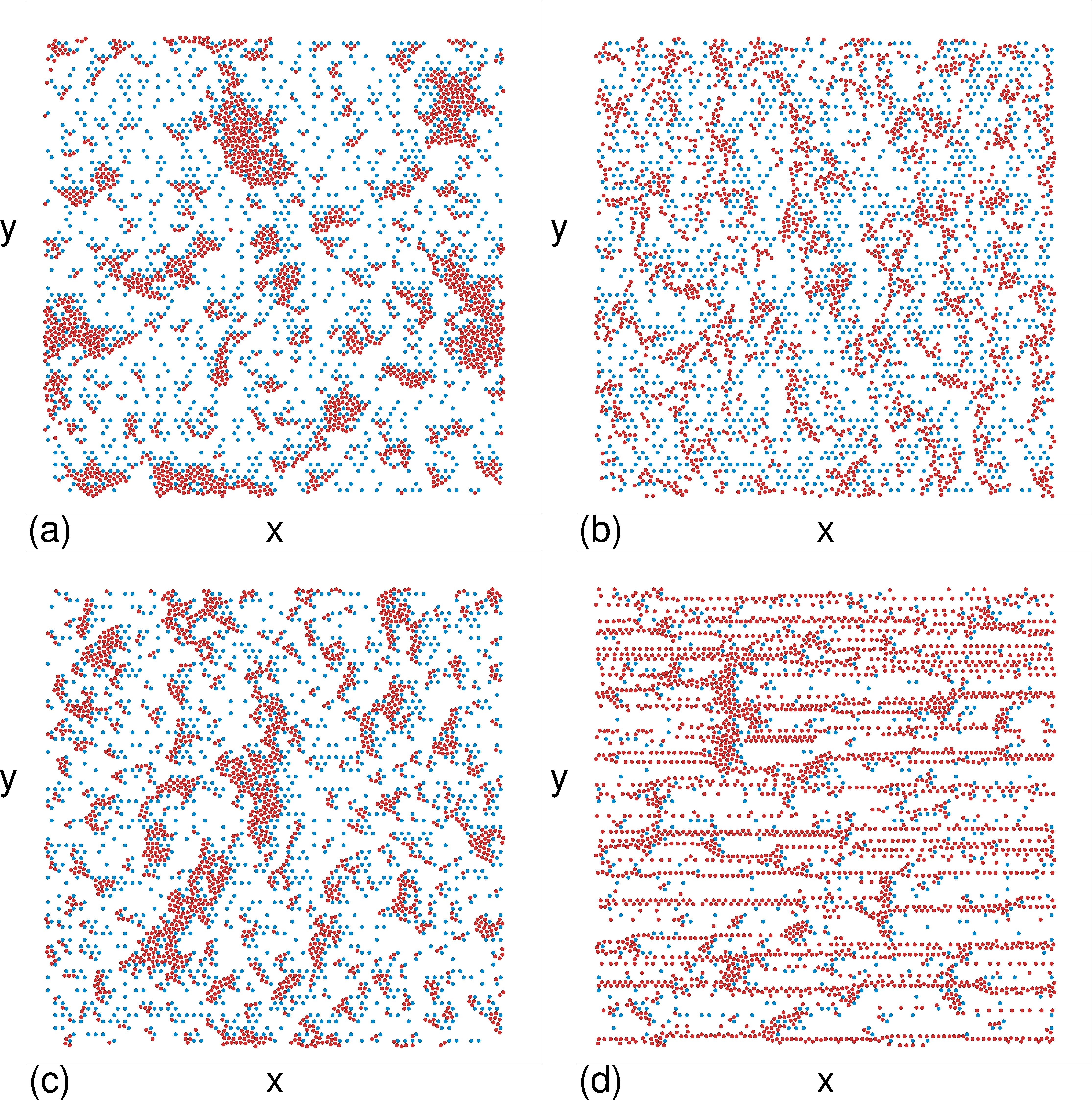
(b) M vs ac frequency ω for the system in Fig. 1(a-c) at ϕtot = 0.275, ϕobs = 0.1256, and Fac = 0.5 for transverse (pink circles) and longitudinal (blue squares) ac driving showing a low frequency clogged state, an intermediate frequency flowing state, and a high frequency clogged state. The letters a, b, c mark the frequencies at which the images in Fig. 1(a-c) were obtained. (c) M vs Fac for the system in (b) under transverse driving with ω = 10−4 (blue), 10−3 (green), 10−2 (gold), and 10−1 (red). (d) M vs Fac|| at the same frequencies as in (c) under longitudinal driving.
In Fig. 2(a) we plot M versus obstacle density ϕobs for a system with ϕtot = 0.275 for zero ac drive, a transverse ac drive of Fac = 0.5 at ω = 10−4, and a transverse dc drive with F||ac=0.5 and ω = 10−4. A clogged state with M=0 appears for ϕtot > 0.115 under no ac drive, for ϕtot > 0.2 under transverse ac driving, and for ϕtot > 0.155 under longitudinal driving. For ϕobs < 0.07, the transverse ac drive produces a slightly lower mobility M than either the longitudinal or zero ac driving. In the inset of Fig. 3(a) we plot a dynamic phase diagram as a function of ϕobs versus ϕtot highlighting the regime with M = 0.0 for the zero ac drive limit (lower line) and for samples with Fac = 0.275 and ω = 10−4 (upper line). In the green shaded area between the two lines, the ac drive unclogs the system. At high ϕtot, both thresholds decrease when the system approaches the crystallization or jamming transition that occurs near ϕtot = 0.9. The images in Fig. 1(a,b,c) are from the ac unclogged region at ϕtot = 0.275 and ϕobs=0.1256, while the image in Fig. 1(d) is from a region that is always unclogged. The extent of the ac unclogged region depends on the ac frequency, and for the highest frequencies, the ac unclogged region decreases in width until both clogging curves coincide.
In Fig. 2(b) we plot M versus ac frequency ω for the system from Fig. 1(a-c) with ϕtot = 0.275 and ϕobs = 0.1256 for transverse and longitudinal ac driving of magnitude Fac=0.5. We find a low mobility state for ω < 10−6 and a zero mobility state for ω ≥ 10−2. The optimal mobility occurs at a frequency of ω ≈ 2.5 ×10⁻⁴. Both directions of ac driving produce the same dynamic states, but the maximum value of M for longitudinal driving is less than half that found for transverse driving, and the window of unclogged states is narrower for longitudinal driving. Additionally, the low frequency states with ω < 10−5 are fully clogged with M = 0 for longitudinal driving, but have a small finite mobility for transverse driving. These results indicate that there are two different types of clogged states separated by an intermediate fluidized state in which the mobility reaches its optimum value. The results in Fig. 2(b) also indicate that there is a wide range of frequencies over which the transverse ac drive is more effective than the longitudinal ac drive at reducing clogging.
In Fig. 2(c) we plot M versus Fac for a system with ϕtot = 0.275 and ϕobs = 0.1256 at the optimal frequency of ω = 10−4 and at ω = 10−3, 10−2, and 10−1. For each driving frequency, there is an optimal value of Fac that maximizes M. Figure 2(d) shows M versus F||ac for the same system at the same driving frequencies. At ω = 10−4, M initially increases with F||ac but it then decreases for ω = 5×10⁻³ until the system reaches a clogged state with M = 0 for F||ac > 1.5. Previous studies of particles moving over randomly placed obstacles under a purely dc drive have shown that negative differential conductivity or a zero mobility state can appear at high dc drives [39,40,41,42]. In our system we find a similar effect under large longitudinal ac drives, so that in general the system reaches a clogged state for high F||ac. For ω = 10−3 in Fig. 2(d), M increases monotonically over the range of F||ac shown; however, M does decrease for much larger values of F||ac. In general, M is higher for transverse ac driving since the transverse shaking permits the particles to more easily move around obstacles, whereas for longitudinal ac driving, the particles are pushed toward the obstacles and M is reduced.
Fig3.png
Figure 3: (a) M vs ϕtot for ϕobs = 0.1256 and Fac = 0.5 at ω = 5.0×10⁻⁶ (blue squares), 10−4 (green circles), 10−2 (pink diamonds) and 10−1 (magenta triangles). Over the entire range of ϕtot, the ω = 10−4 curve has the highest values of M. Inset: dynamic phase diagram as a function of ϕobs vs ϕtot. Circles indicate the clogging threshold for zero ac drive, and squares indicate the clogging threshold under a transverse ac drive with Fac=0.5 and ω = 10−4. Yellow: flowing state. Blue: clogged state. Green: Flowing under ac drive, clogged without ac drive. The letters a to d indicate locations at which images in Fig. 1(a-d) were obtained. (b) M vs ϕtot in the same system for transverse (green circles) and longitudinal (red squares) ac driving at ω = 10−4, where transverse ac driving produces the highest values of M.
In Fig. 3(a) we plot M versus ϕtot for samples with ϕobs = 0.1256 and Fac = 0.5 at ω = 5.0×10⁻⁶, 10−4, 10−2, and 10−1. M is always small at low ϕtot, increases to a local maximum at ϕtot = 0.5, and decreases to zero as ϕtot approaches ϕtot=0.85, corresponding to the density at which the system starts to form a crystallized solid state [38,43]. We find the highest mobility for ω = 10−4, particularly for 0.66 < ϕtot < 0.85 where M is close to zero for ω = 10−2 and 10−1. In Fig. 3(b) we show M versus ϕtot at ω = 10−4 for transverse and longitudinal ac driving, where we again find that the transverse ac driving gives higher values of M for all ϕtot and where the local maximum in M falls at ϕtot = 0.5 for both ac driving directions. The M versus ϕtot curve has a maximum near ϕ = 0.5 and goes to zero at both high and low ϕtot, following the clogging behavior of the phase diagram in the inset of Fig. 3(a). The results in Fig. 3(a) show slices through the phase diagram at constant ϕobs = 0.1256 and varied ϕtot within the ac unclogged region where the clogging is fragile against application of an ac drive.
Fig4.png
Figure 4: (a) M vs ω for samples with ϕtot = 0.275 and Fac = 0.5 at ϕobs = 0.00157, 0.031416, 0.047124, 0.062831, 0.07754, 0.09424, 0.1099, 0.1256 [also shown in Fig. 2(b)], 0.14137, and 0.157, from top to bottom. (b) Dynamic phase diagram as a function of ϕobs vs ω for transverse driving with Fac=0.5. I: flowing fluidized state; II: creeping clogged state; III: frozen clogged state.
In Fig. 4(a) we plot M versus ω in samples with ϕtot=0.275 and Fac=0.5 at ϕobs = 0.00157 to 0.157, which also includes the curve from Fig. 2(b) at ϕobs = 0.256. For ϕobs > 0.1099, the system reaches a fully clogged state with M = 0. We define the onset of the low frequency clogged state as the point at which M < 0.02. A local maximum in M appears near ω = 2.5 ×10⁻⁴ and shifts to slightly lower frequencies as ϕobs decreases. A local minimum near ω = 10−3 develops when ϕobs < 0.1099, and this minimum also shifts to lower frequencies with decreasing ϕobs. Both of the local extrema are correlated with characteristic length scales of the system. The local maximum at ϕobs = 0.1256 falls at a value of ω for which the distance dτ−1dt(Fac/√2+Fdc) a particle moves during a single ac cycle matches the average spacing 1/√{ϕobs} between obstacles. As this average spacing decreases for increasing ϕobs, the frequency at which the maximum value of M occurs decreases as well. The frequency at which the local minimum appears for ϕobs < 0.1099 corresponds to the point at which dτ matches the minimum transverse surface-to-surface obstacle spacing of dmin−2Rd. At this matching frequency, the particles preferentially collide with the obstacles rather than moving between them or around them, reducing the mobility. The two resonant frequencies are separated by a factor of 10 since Fac/Fdc = 10.
In Fig. 4(b) we plot a dynamic phase diagram as a function of ϕobs versus ω for samples with Fac=0.5. Here phase I is the flowing fluidized state, phase II is the low frequency creeping clogged state, and phase III is the frozen clogged state. For ϕobs > 0.165, the spacing between obstacles becomes so small that the system is in a frozen state for all values of ω. The fluidized state is of maximum extent between ω = 10−5 and ω = 10−4. The dynamic phase diagram for longitudinal ac driving (not shown) is similar; however, the extent of phase I is reduced. The results in Fig. 4(b) are partially obtained from the curves in Fig. 4(a). At higher densities the optimal frequency corresponds to where the ac drive can unclog the system, while at lower obstacle densities where the system is always in phase I, the regimes of lower mobility represent a vestige of the high and low frequency clogging behaviors from phases II and III.
Our results resemble what has been found in recent experiments on the viscosity of vibrated granular matter, where the system is in a jammed state for low vibration frequencies, enters a low viscosity fluid state at intermediate frequencies, and shows a reentrant jammed state at high frequencies [37]. Other studies have also revealed optimal frequencies for dynamic resonances in granular matter, where the speed of sound is the lowest at intermediate frequencies when the grains are the least jammed [44].

Summary

We have examined the clogging and flow of particles moving through random obstacle arrays under a dc drift and an additional transverse or longitudinal ac drive. At zero ac driving, there is a well defined obstacle density above which the system reaches a clogged state. When ac driving is added, this clogging transition shifts to much higher obstacle densities. For large obstacle densities, we find a low frequency creeping clogged state where the particles undergo rearrangements from one clogged configuration to another with a drift mobility that is nearly zero. At intermediate frequencies, the particles form a high mobility fluidized state, while at high frequencies, a zero mobility frozen clogged state appears, so that there is an optimal mobility at intermediate frequencies. The mobility is also nonmonotonic as a function of ac driving amplitude for fixed ac driving frequency. In most cases the transverse ac driving is more effective at increasing the mobility than longitudinal ac driving. When the ac amplitude and frequency are both fixed, we find that there is an optimal disk density that maximizes the mobility, while for high disk densities the system enters a low mobility jammed state. At low obstacle densities the system is always in a flowing state; however, for transverse ac driving we find a resonant frequency with reduced flow when the magnitude of the transverse oscillations matches the minimum transverse spacing of the obstacles. We map a dynamic phase diagram showing the locations of the flowing state, creeping clogged state, and frozen clogged state.
Our results suggest that ac driving could be used to avoid clogging and to optimize particle flows in disordered media, and this technique could also be used as a method for separating different species of particles, where different species could have different mobilities as a function of frequency so it would possible one spices clogged and the other mobile.. Our results can be generalized for controlling flows in a wide class of collectively interacting particle systems in heterogeneous environments, including colloids, bubbles, granular matter, vortices in superconductors, and skyrmions in chiral magnets.
We gratefully acknowledge the support of the U.S. Department of Energy through the LANL/LDRD program for this work. This work was carried out under the auspices of the NNSA of the U.S. DoE at LANL under Contract No. DE-AC52-06NA25396 and through the LANL/LDRD program.

References

[1]
L.M. McDowell-Boyer, J.R. Hunt, and N. Sitar, Water Resour. Res. 22, 1901 (1986).
[2]
D.C. Mays and J.R. Hunt, Environ. Sci. Technol. 39, 577 (2005).
[3]
L.R. Huang, E.C. Cox, R.H. Austin, and J.C. Sturm, Science 304, 987 (2004).
[4]
P. Tierno, T.H. Johansen, and T.M. Fischer, Phys. Rev. Lett. 99, 038303 (2007).
[5]
Z. Li and G. Drazer, Phys. Rev. Lett. 98, 050602 (2007).
[6]
R. Zhang and J. Koplik, Phys. Rev. E 85, 026314 (2012).
[7]
J. McGrath, M. Jimenez, and H. Bridle, Lab Chip 14, 4139 (2014).
[8]
H.M. Wyss, D.L. Blair, J.F. Morris, H.A. Stone, and D.A. Weitz, Phys. Rev. E 74, 061402 (2006).
[9]
F. Chevoir, F. Gaulard, and N. Roussel, Europhys. Lett. 79, 14001 (2007).
[10]
G.C. Agbangla, P. Bacchin, and E. Clement, Soft Matter 10, 6303 (2014).
[11]
H. T. Nguyen, C. Reichhardt, and C.J.O. Reichhardt, Phys. Rev. E 95, 030902(R) (2017).
[12]
H. Peter, A. Libal, C. Reichhardt, and C.J.O. Reichhardt, Sci. Rep. 8, 10252 (2018).
[13]
R.L. Stoop and P. Tierno, arXiv:1712.05321.
[14]
S. Redner and S. Datta, Phys. Rev. Lett. 84, 6018 (2000).
[15]
N. Roussel, T. L. H. Nguyen, and P. Coussot, Phys. Rev. Lett. 98, 114502 (2007).
[16]
C. Barré and J. Talbot, J. Stat. Mech. 2017, 043406 (2017).
[17]
O. Chepizhko, E.G. Altmann, and F. Peruani, Phys. Rev. Lett. 110, 238101 (2013).
[18]
C. Bechinger, R. Di Leonardo, H. Löwen, C. Reichhardt, G. Volpe, and G. Volpe, Rev. Mod. Phys. 88, 045006 (2016).
[19]
A. Morin, N. Desreumaux, J.-B. Caussin, and D. Bartolo, Nat. Phys.13 , 63 (2017).
[20]
Cs. Sándor, A. Libál, C. Reichhardt, and C.J.O. Reichhardt, Phys. Rev. E 95, 032606 (2017).
[21]
C. Reichhardt and C.J.O. Reichhardt, Rep. Prog. Phys 80, 026501 (2017).
[22]
K. To, P.-Y. Lai, and H. K. Pak, Phys. Rev. Lett. 86, 71 (2001).
[23]
I. Zuriguel, L. A. Pugnaloni, A. Garcimartín, and D. Maza, Phys. Rev. E 68, 030301(R) (2003).
[24]
D. Chen, K. W. Desmond, and E. R. Weeks, Soft Matter 8, 10486 (2012).
[25]
I. Zuriguel et al., Sci. Rep. 4, 7324 (2014).
[26]
R. C. Hidalgo, A. Goñi-Arana, A. Hernández-Puerta, and I. Pagonabarraga, Phys. Rev. E 97, 012611 (2018).
[27]
C. Mankoc, A. Garcimartín, I. Zuriguel, D. Maza, and L. A. Pugnaloni, Phys. Rev. E 80, 011309 (2009).
[28]
C. Lozano, G. Lumay, I. Zuriguel, R. C. Hidalgo, and A. Garcimartín, Phys. Rev. Lett. 109, 068001 (2012).
[29]
A. Janda, D. Maza, A. Garcimartín, E. Kolb, J. Lanuza, and E. Clément, Europhys. Lett. 87, 24002 (2009).
[30]
J.A. Dijksman, G.H. Wortel, L.T.H. van Dellen, O. Dauchot, and M. van Hecke, Phys. Rev. Lett. 107, 108303 (2011).
[31]
M. Griffa, E. G. Daub, R. A. Guyer, P. A. Johnson, C. Marone, and J. Carmeliet, Europhys. Lett. 96, 14001 (2011).
[32]
H. Lastakowski, J.-C. Géminard, and V. Vidal, Sci. Rep. 5, 13455 (2015).
[33]
K. To and H.-T. Tai, Phys. Rev. E 96, 032906 (2017).
[34]
G. A. Patterson, P. I. Fierens, F. Sangiullano Jimka, P. G. König, A. Garcimartín, I. Zuriguel, L. A. Pugnaloni, and D. R. Parisi, Phys. Rev. Lett. 119, 248301 (2017).
[35]
D. Helbing, I.J. Farkas, and T. Vicsek, Phys. Rev. Lett. 84, 1240 (2000).
[36]
J.M. Pastor, A. Garcimartín, P.A. Gago, J.P. Peralta, C. Martín-Gómez, L.M. Ferrer, D. Maza, D.R. Parisi, L.A. Pugnaloni, and I. Zuriguel, Phys. Rev. E 92, 062817 (2015).
[37]
A. Gnoli, L. de Arcangelis, F. Giacco, E. Lippiello, M.P. Ciamarra, A. Puglisi, and A. Sarracino, Phys. Rev. Lett. 120, 138001 (2018).
[38]
C. Reichhardt and C.J.O. Reichhardt, Soft Matter 10, 2932 (2014).
[39]
S. Leitmann and T. Franosch, Phys. Rev. Lett. 111, 190603 (2013).
[40]
U. Basu and C. Maes, J. Phys. A: Math. Theor. 47, 255003 (2014).
[41]
O. Bénichou, P. Illien, G. Oshanin, A. Sarracino, and R. Voituriez, Phys. Rev. Lett. 113, 268002 (2014).
[42]
M. Baiesi, A.L. Stella, and C. Vanderzande, Phys. Rev. E 92, 042121 (2015).
[43]
A. J. Liu and S. R. Nagel, Annu. Rev. Condens. Matter Phys. 1, 347 (2010).
[44]
C.J.O. Reichhardt, L.M. Lopatina, X. Jia, and P.A. Johnson, Phys. Rev. E 92, 022203 (2015).


File translated from TEX by TTHgold, version 4.00.
Back to Home