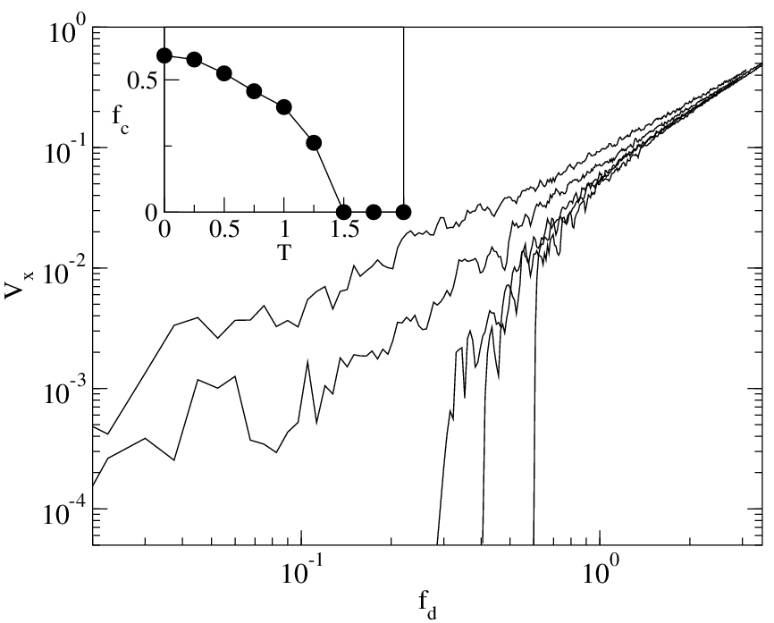
 Figure 5:
The velocity Vx vs fd for a single driven probe particle for
T = 3.5, 2.0, 1.25, 1.0, and 0 from left to right.
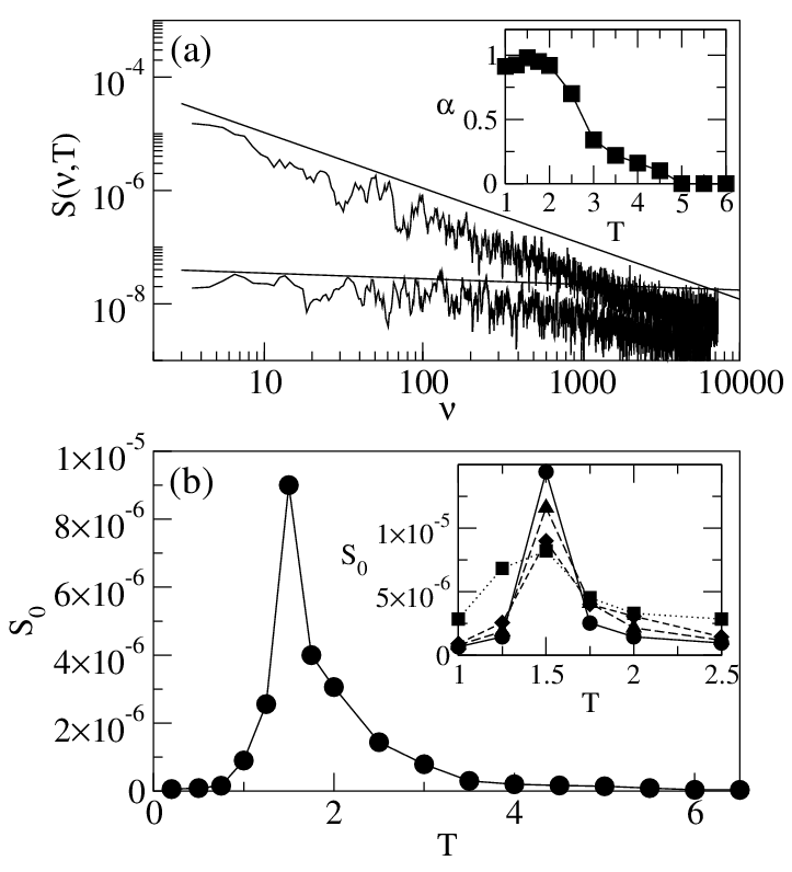
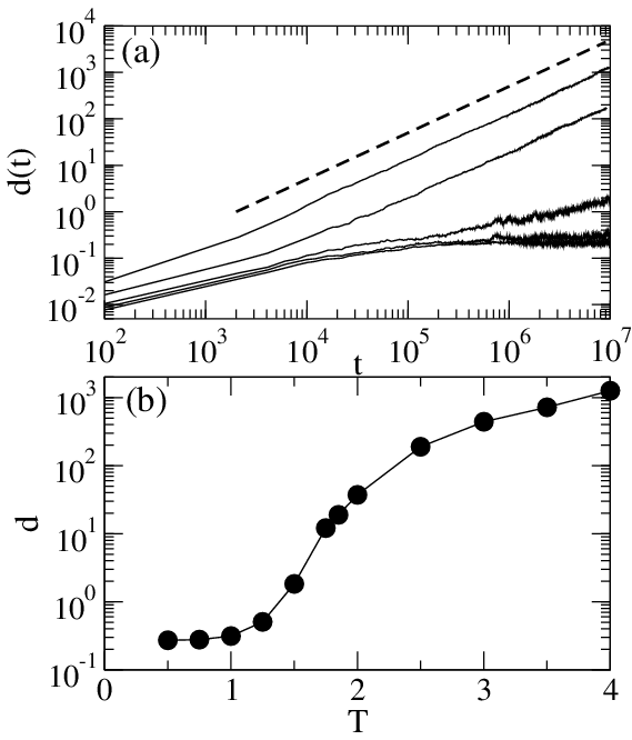
The peak
in the noise power of the defect fluctuation power spectra occurs
at T = Tn = 1.5, which also corresponds to the onset of the subdiffusive
motion.
Inset: the
threshold force fc extracted from the velocity-force curves
vs T.
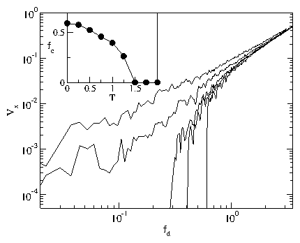
Figure 5:
The velocity Vx vs fd for a single driven probe particle for
T = 3.5, 2.0, 1.25, 1.0, and 0 from left to right.
The peak
in the noise power of the defect fluctuation power spectra occurs
at T = Tn = 1.5, which also corresponds to the onset of the subdiffusive
motion.
Inset: the
threshold force fc extracted from the velocity-force curves
vs T.
|