| in1 | in2 | in3 | out |
| 0 | 0 | 0 | 0 |
| 0 | 0 | 1 | 1 |
| 0 | 1 | 0 | 1 |
| 0 | 1 | 1 | 0 |
| 1 | 0 | 0 | 0 |
| 1 | 0 | 1 | 1 |
| 1 | 1 | 0 | 0 |
| 1 | 1 | 1 | 1 |
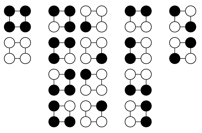
| in | |||||||||||||||||||
| 00 | 0 | 1 | 0 | 1 | 0 | 1 | 1 | 0 | 0 | 0 | 0 | 1 | 1 | 1 | 1 | 0 | |||
| 01 | 0 | 1 | 0 | 1 | 1 | 0 | 0 | 1 | 0 | 0 | 1 | 0 | 1 | 1 | 0 | 1 | |||
| 10 | 0 | 1 | 1 | 0 | 0 | 1 | 0 | 0 | 1 | 0 | 1 | 1 | 0 | 1 | 0 | 1 | |||
| 11 | 0 | 1 | 1 | 0 | 1 | 0 | 0 | 0 | 0 | 1 | 1 | 1 | 1 | 0 | 1 | 0 | |||
| P0 | 1 | 1 | 0 | 0 | 0 | 0 | 0 | 0 | 0 | 0 | 0 | 0 | 0 | 0 | 0 | 0 | |||
| P1 | 1 | 1 | [1/2] | [1/2] | [1/2] | [1/2] | [1/2] | [1/2] | [1/2] | [1/2] | [1/2] | [1/2] | [1/2] | [1/2] | 0 | 0 | |||
|
|
|
| (1) |
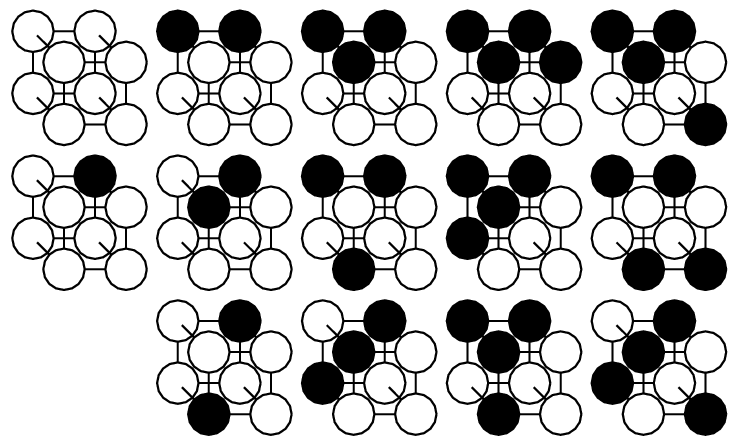
| k | Cycle polynomial | PG |
| 1 | (1/2)(x12+x2) | 2 |
| 2 | (1/8)(x14+3x22+2x12x2+2x4) | 4 |
| 3 | (1/48)(x18+13x24+8x12x32+8x2x6+6x14x22+12x42) | 14 |
| 4 | (1/384)(x116+12x18x24+51x28+12x14x26+32x14x34+48x12x2x43+84x44 | |
| +96x22x62+48x82) | 238 | |
| 5 | (1/3840)(x132+384x103x2+20x116x28+60x18x212+231x216+80x18x38 | |
| +320x122x42+240x14x22x46+240x24x46+520x48+384x12x56 | ||
| +160x14x22x34x62+720x24x64+480x84) | 698635 | |
| (2) |
| Class type | Nh | 〈Sc〉 |
| A4 | 1 | 2 |
| A3B | 1 | 8 |
| A2B2 | 2 | 3 |
| Class type | Nh | 〈Sc〉 |
| A8 | 1 | 2 |
| A7B | 1 | 16 |
| A6B2 | 3 | 18.667 |
| A5B3 | 3 | 37.333 |
| A4B4 | 6 | 11.667 |
| Class type | Nh | 〈Sc〉 |
| A16 | 1 | 2 |
| A15B | 1 | 16 |
| A14B2 | 4 | 60 |
| A13B3 | 6 | 186.667 |
| A12B4 | 19 | 191.58 |
| A11B5 | 27 | 323.56 |
| A10B6 | 50 | 320.32 |
| A9B7 | 56 | 408.57 |
| A8B8 | 74 | 173.9 |
| Class type | Nh | 〈Sc〉 |
| A32 | 1 | 2 |
| A31B | 1 | 64 |
| A30B2 | 5 | 198.4 |
| A29B3 | 10 | 992 |
| A28B4 | 47 | 1530.2 |
| A27B5 | 131 | 3074.4 |
| A26B6 | 472 | 3839.8 |
| A25B7 | 1326 | 5076.7 |
| A24B8 | 3779 | 5566.7 |
| A23B9 | 9013 | 6224.1 |
| A22B10 | 19963 | 6463.2 |
| A21B11 | 38073 | 6777.7 |
| A20B12 | 65664 | 6877.2 |
| A19B13 | 98804 | 7031.6 |
| A18B14 | 133576 | 7058.7 |
| A17B15 | 158658 | 7131.3 |
| A16B16 | 169112 | 3554.3 |
| (3) |

|
| (4) |
| (5) |