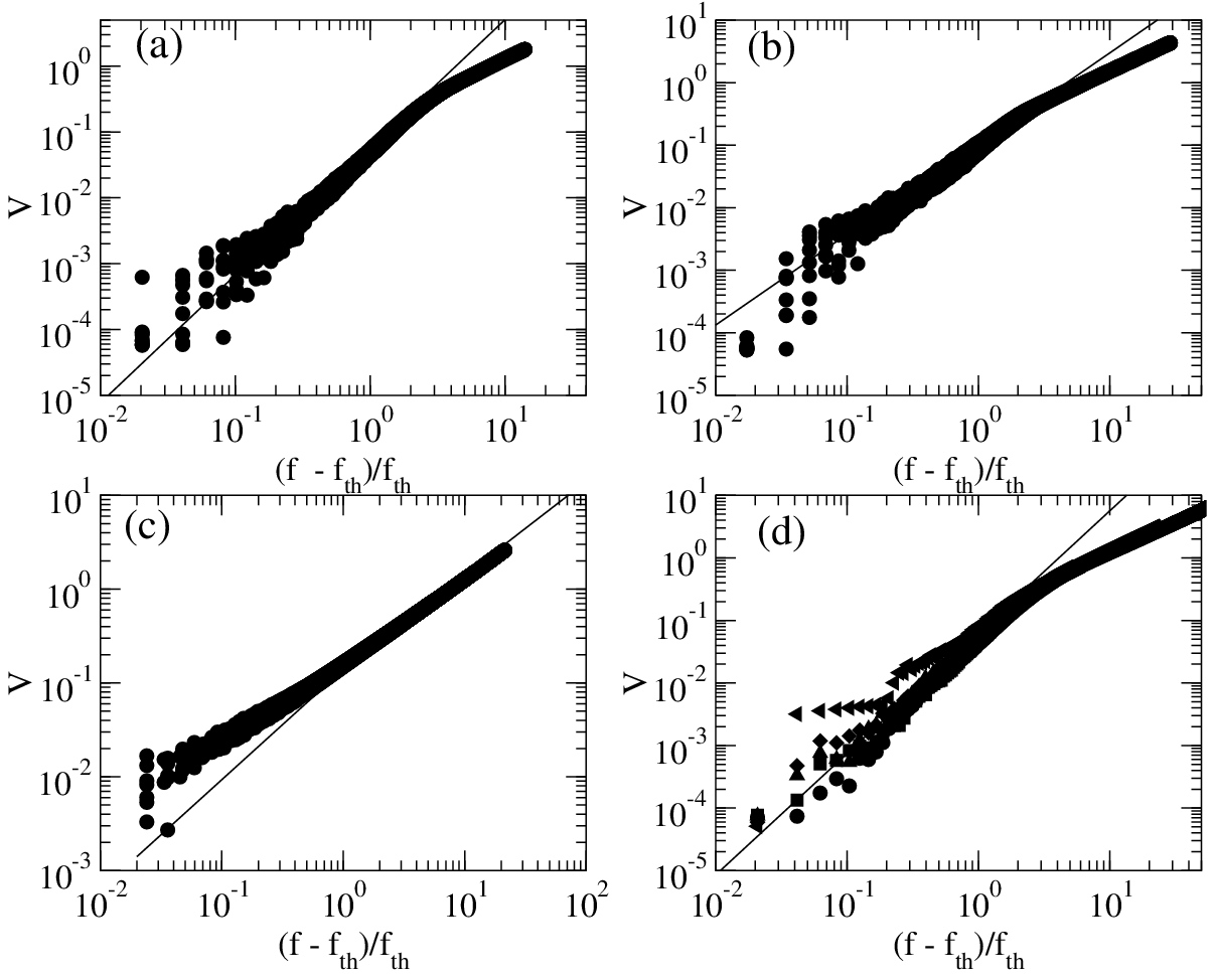
Physical Review Letters 90, 046802 (2003)

Charge Transport Transitions and Scaling in Disordered Arrays of Metallic Dots

C. Reichhardt and C.J. Olson Reichhardt

Center for Nonlinear Studies and Theoretical Division, Los Alamos National Laboratory, Los Alamos, New Mexico 87545

(Received 25 May 2002; published 28 January 2003)

We examine the charge transport through disordered arrays of metallic dots using numerical simulations. We find power law scaling in the current-voltage curves for arrays containing no voids, while for void-filled arrays charge bottlenecks form and a single scaling is absent, in agreement with recent experiments. In the void-free case we also show that the scaling exponent depends on the effective dimensionality of the system. For increasing applied drives we find a transition from 2D disordered filamentary flow near threshold to a 1D smectic flow which can be identified experimentally using characteristics in the transport curves and conduction noise.
A wide variety of disordered systems exhibit threshold behavior and nonlinear response to an applied drive. Examples include flux lines in disordered superconductors, [1,2,3] charge-density-waves (CDW's) pinned by impurities [4], Wigner crystals [5,6] in semiconductors with charge impurities, and colloids flowing over rough surfaces [7]. Another example is charge transport through metallic dot arrays. Middleton and Wingreen (MW) have considered a model of this system in which the randomly charged dots are separated by tunnel barriers [8]. They found threshold behaviors and scaling of the current-voltage curves of the form I = (V/VT − 1)ζ. In 1D they obtain ζ = 1.0, while for 2D they predict analytically ζ = 5/3 and find in simulations ζ = 2. For the 2D systems the simulated flow patterns are not straight but form intricate meandering paths with considerable transverse fluctuations. These same types of meandering paths are also observed in the flow of flux-lines [1,3], Wigner crystals [6], and colloids [7] above the depinning threshold. Experimental studies in metal dot arrays have also found scaling in the I-V curves for 2D and 1D systems [9,10,11,12,13]; however, the scaling exponents in these experiments exhibit a wide range of values. The studies for 1D arrays [9] find a scaling exponent of ζ = 1.36, which is less than the value for 2D arrays predicted by MW, but still larger than the expected 1D value of ζ = 1.0. It is not known if this system is truly 1D, or whether some meandering of the charge in 2D can still occur due to the finite width of the dots. It is also not known how the exponents would change (or whether there would even be scaling) upon changing the system from 2D to 1D by gradually narrowing the array width. Other systems in 2D exhibiting scaling near depinning also show a wide spectrum of scaling exponents [1,2,3,6,7], suggesting that the type of disorder and the effective dimensionality of the array plays a crucial role in the transport.
Recently, to address the role of different types of disorder on transport, Parthasarathy et al. [14] have performed experiments on triangular monolayers of gold nanocrystals. Disorder is present in the form of charge disorder in the substrate as well as variations in the interparticle couplings. Structural disorder was also introduced by creating voids in the arrays. The void-free arrays exhibit robust power law scaling with ζ = 2.25. A single power law could not be fit for the structurally disordered arrays. Parthasarathy et al. conjecture that in arrays with voids, the charge must be shuttled into bottleneck regions which reduces the amount of charge flow. In the theoretical studies of MW where structural disorder was not considered, only power law behavior was observed [8].
Since the charge flow at depinning in the dot arrays resembles that seen in other systems such as flux lattices, it is of interest to ask whether some of the ideas developed in these other systems can be carried over to the metallic dot system. In disordered vortex systems, theory [15,16,17], simulation [15,18], and experiment [19] show that at low drives the vortex flow is highly disordered, meanders in 2D, and the overall lattice structure is destroyed. For high drives there can be a remarkable reordering transition where the flow occurs in 1D channels and the lattice regains considerable order. For strong quenched disorder in 2D, the highly driven phase forms a moving smectic with order in the transverse but not the longitudinal direction. Here the vortices move in well spaced channels, and the channels are decoupled from one another.
In order to compare to the recent experiments and to explore the points raised above, we conduct molecular dynamics simulations of a simple model for charge transport in 2D arrays with charge disorder and both with and without structural order. In our model we consider square and rectangular arrays of side N×M, with periodic boundary conditions in the x and, for the 2D systems, y directions, containing Nc mobile charges. A charge i follows the overdamped equation of motion, fivi = −∑jNcU(rij) + fd + fp. The mobile charges interact via a long-range Coulomb term, U = q2/r, which we treat with a summation technique [20] for numerical efficiency. Under an applied drive fd = fdx, a mobile charge on a site, represented by a parabolic trap, experiences a maximum threshold force fp=fth before exiting the plaquette. For actual dot arrays the applied drive comes from an applied voltage V, and the energy to add an electron to a dot with charge q is Vth = q/C where C is the capacitance of the dot. Charge flow will then occur for applied drives V > Vth for a single dot. For arrays without voids, we add disorder by selecting random thresholds Vth from a Gaussian distribution centered at V0th. To study the effect of structural disorder, a portion P < 0.5 of randomly selected sites is effectively voided by setting Vth to a very large value so that mobile charge cannot flow through them. We do not consider thermal effects since our system is in the Coulomb-blockade regime, so that charging energies are higher than the thermal energies. For increasing applied drive or voltage we measure the global charge flow or current I=Vx=(1/Nc)∑vi ·x. We also measure the trajectories of the flow and the fluctuations in the current, which is proportional to the conduction noise.
Fig1.png
Figure 1: 
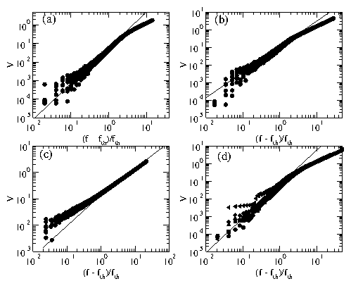
The scaling of the average velocity V vs applied drive f for (a) a 2D system with a fit of ζ = 1.94 (solid line) with nine disorder realizations and (b) a system of dimension 5 ×500 with a ζ = 1.45 fit (solid line), for eight disorder realizations. fth is the threshold force at which depinning occurs. (c) A system geometry of 1 ×500, showing a fit with ζ = 1.0 (solid line) for nine disorder realizations. (d) 2D systems for sizes 16 ×16 (triangle left), 30 ×30 (triangle up), 38 ×38 (diamond), 50 ×50 (square), and 60 ×60 (circle). The solid line is a ζ = 1.94 fit.
We first consider the scaling for ordered arrays in 2D, 1D, and finite width samples. In Fig. 1(a) we show the scaling of the average flow vs applied drive (I-V) curves for the 2D case for nine disorder realizations, and in Fig. 1(c) the 1D case. For 2D we find scaling with ζ = 1.94 ±0.15 in fair agreement with the simulation results ζ = 2.0 of MW, but still lower than the ζ = 2.25 found in Ref. [14] for ordered arrays. The simulations for 1D give a linear behavior for much of the curve, suggesting that if a scaling exponent could be ascribed it would be ζ < 1.0; however, for drives near threshold, a single scaling cannot be applied and the curve bends up. We note that for the depinning of 1D elastic objects such as CDW's one expects an exponent of ζ = 1/2 [4]. Experiments measuring the threshold of a single dot also find ζ = 1/2 [10]. Fig. 1(c) shows that the deviation from linearity occurs only very near threshold, so that the discrepancy between our results and MW may result from MW not being close enough to the threshold to see the deviation. In Fig. 1(b) the scaling for a wider system of 5×500 with eight disorder realizations is shown, where we find scaling with ζ = 1.45 ±0.08. We note that experiments for the 1D arrays [10] find ζ = 1.36. Our results suggest that scaling can occur for systems between 1 and 2 dimensions with the value of the exponent monotonically increasing from 1/2 in 1D to 2.0 in 2D. We have also simulated system sizes of 2×500 and find linear scaling similar to the 1D case. Additional evidence for the increase of the exponent as a function of dimensionality has been obtained in cobalt nanocrystal samples of finite thickness, with an effective dimensionality between 2 and 3. Here exponents of 2.2 < ζ < 2.7 are observed [12]. Our results also suggest that the experiment in [14] is in an effective dimension higher than 2.0. All of the curves in Fig. 1 show a crossover to a linear regime at high drives, which was also seen in the earlier numerical work. We find no hysteresis for either the 2D or 1D case.
In Fig. 1(d) we consider the 2D case for different system sizes ranging from 16 ×16 up to 60 ×60. The exponent does not change for the larger systems, indicating that our systems are large enough to capture the correct exponent for the model considered here. Only the smallest system (16 ×16) shows significant deviation. We have also simulated different system sizes for the 1D and quasi-1D case and find similar results. We note that much larger systems would be needed to approach the typical experimental sizes. The rate at which the applied drive is increased can also affect the measured exponents. At rapid sweep rates, transient states rather than steady states appear, and both the measured current and the apparent exponents are larger than the steady state values. All our results are from a steady state.
Fig2.png
Figure 2: The current paths for increasing applied drives in the 2D system shown in Fig. 1(a). Here (a) fd/fth = 1.1 and (b) fd/fth = 2.0 produce meandering 2D channels. In (c) fd/fth = 10.0 produces straight 1D channels.
We next consider the flow transitions for increasing applied drive in the 2D system. In Fig. 2 we show the current paths for three different applied drives above threshold. In Fig. 2(a), at fd/fth = 1.1 the flow follows meandering paths in only a few regions of the sample, in agreement with the simulations of MW [8]. These flow paths are stationary over time. For higher drives, as seen in Fig. 2(b) at fd/fth = 2.0, there is a crossover from the static paths to dynamic paths which open, close, and shift position over time. The filamentary flow in this case occurs everywhere in the system over time. For drives at and above the fd value where the I-V curve becomes linear, as seen in Fig. 2(c) for fd/fth = 10.0, there is a crossover from the meandering 2D flow to straight 1D ordered channels of flow. Fig. 2(c) shows that the charge moves only in 1D channels without any jumping of charge between adjacent channels. The channels themselves carry different amounts of flowing charge due to the different average disorder along the rows. The charges in one channel do not synchronize with the flow of charge in adjacent channels; instead, the channels slide past one another. We term this a smectic flow state since the channels are periodically spaced in the transverse direction but are independently moving in the longitudinal direction. The transition from the disordered to partially ordered flow is very similar to the reordering transitions seen for driven vortex lattices [15,16,17,18,19]. We observe the same transitions in the systems of finite widths.
Fig3.png
Figure 3: (a) Circles: dV/df of the curve shown in Fig. 1(a) for a 2D system. Squares: The noise power S0 as a function of drive. (b) Consecutive power spectra for increasing fd for, from bottom to top, fd/fth = 1.1, 2.0, 5.0, and 8.0. The curves have been shifted up for presentation.
In Fig. 3(a) we plot the dV/df curve, which is proportional to the resistance R, for the 2D system in Fig. 1(a). The crossover to the linear regime (with constant R) appears as the plateau region in dV/df. Also shown in Fig. 3(a) is the power S0 from one octave of the power spectra of the conduction noise at four different applied drives fd: S0=∫ν1ν2 dνS(ν), where S(ν) = |∫Vx(t)ei2πνtdt|2. The noise power shows a peak in the scaling regime near fd=0.35 and then decreases in the linear regime with a low value of S0 during the smectic flow. In Fig. 3(b) we show that a clearer signature of the flow phases can be obtained by examining individual power spectra. For drives in the scaling regime we find a 1/fα power spectra, which is indicative of the many different frequencies generated by the complex flow patterns illustrated in Fig. 2(a,b). The large noise power and 1/fα signals have also been associated with meandering disordered flow in superconducting vortices. For increasing drive a characteristic peak in the spectra begins to appear and is most prominent in the smectic flow regime. This peak occurs when the charge in the smectic phase flows in 1D paths along the dots which are in a periodic array of spacing a. The frequency at which the peak occurs is then ν = v/a, where v is the average velocity of the charge. For perfectly ordered flow, the peaks would be very narrow. Since the channels have different amounts of flowing charge there is some dispersion in the frequency. The presence of peaks in the power spectra suggests that it would be possible to observe an interference effect, or Shapiro steps, in the I-V curves if an additional applied AC drive is imposed with a frequency that matches the frequency of the system.
Another experimental probe of the moving smectic phase is the presence of a transverse depinning barrier as first predicted in [17] for elastic media. If a transverse force is applied to the already longitudinally moving system, then in the disordered regime there is no threshold for transverse motion and some charge will immediately begin to move in the transverse direction. For the high drive regime, after the 1D moving channels have formed, there is a finite transverse threshold since the channels are effectively pinned in the transverse direction. There may also be interesting results for driving along different directions of the dot lattice. Although there is randomness in the individual dot strength, the overall topological order of the array can break the symmetry so that certain directions may allow easier charge flow than others.
Fig4.png
Figure 4: (a) The average velocity at a fixed fd=0.2 for a system with increasing void fraction P. The solid line is a fit with V = 2(0.5 − P)1.5. (b) The velocity vs applied drive curve for a void fraction of P=0.47. (c) The trajectories for a system with a void fraction of P=0.47 at fd/fth = 3.0.
We next consider the structurally disordered arrays. We find that for a fixed applied drive, the current is reduced as the void fraction P is increased. This is understandable since the charges must flow in increasingly winding patterns to pass the voids, which are effective obstacles. In Fig. 4(a) we plot V vs P up to P=0.49 for a fixed fd = 0.2. For the decreasing value of V, we find a best fit to a power law with V = V0(0.5 −P)1.5. The current should go to zero for P = 0.5, or the percolation limit, where for an infinite system voids would span the entire system. In our system there is still transport for P > 0.5 due to finite size effects. In Fig. 4(b) we show the current vs applied drive curve for a void fraction of P=0.47. In this case, we cannot fit a single power law above threshold. In Ref. [14] the additional features in the I-V curves for the structurally disordered arrays were conjectured to occur due to bottleneck effects caused by the void regions. In Fig. 4(c) we illustrate the current paths for fd/fth = 3.0 and P=0.47, showing that there is considerable flow through the system, but that in certain well-defined areas no flow is occurring. Averaging the trajectories over a longer time produces the same flow patterns shown in Fig. 4(c). This is in contrast to the flow pattern in Fig. 2(b), which changes over time, so that for long times flow occurs in all regions of the sample. In Fig. 4(c) some bottlenecks can also be seen in the form of regions where the trajectories are compressed. For the structurally disordered arrays the transition to the smectic flow at higher drives is absent since straight 1D flows cannot occur even in the ohmic regime. The conduction noise shows the same 1/fα behavior as the ordered arrays but the peaks in the noise spectra are absent in the ohmic regime.
Another issue is the possible effect of the edges, which may induce a 1D or quasi 1D correlated region of stronger or weaker disorder. These effects could be particularly relevant for systems of finite width. To test this, we have performed simulations of void-free systems where a correlated 1D region of strong or weak disorder is added to mimic possible edge effects. For the small 2D systems and for systems with small aspect ratios, the I-V curves are very similar to those seen in Fig. 4(b) where a single power law is absent. For the larger systems this effect washes out and the system returns to the pure 2D case.
In summary, we have investigated charge transport in structurally ordered and disordered arrays. For ordered arrays we find scaling in the current vs applied drive curves with ζ = 1.94 in 2D, while for 1D arrays the scaling exponent ζ < 1. Scaling still occurs for systems with finite width, with the exponent increasing toward ζ = 2.0 for increasing sample widths. For increasing applied drive in 2D, we show that the crossover to ohmic behavior coincides with a change in the flow from 2D meandering to straight 1D channels or smectic flow. Evidence for this change in the flow also appears in the form of a crossover in the power spectra, which shows a broad 1/fα signature in the disordered flow regime, and a characteristic peak or washboard signal in the smectic flow regime. For disordered arrays where a fraction of the sites are replaced with voids, a single power law cannot be fit to the I-V curve in agreement with recent experiments. The transition from the 2D disordered flow to the 1D channel flow is absent in the structurally disordered arrays.
We thank A.A. Middleton, H. Jaeger, and R. Parthasarathy for useful discussions. This work was supported by the U.S. Department of Energy under Contract No. W-7405-ENG-36.

References

[1]
H.J. Jensen, A. Brass, Y. Brechet, and A.J. Berlinsky, Phys. Rev. B 38, 9235 (1988).
[2]
S. Bhattacharya and M.J. Higgins, Phys. Rev. Lett. 70, 2617 (1993); Phys. Rev. B 49, 10005 (1994); M. Danckwerts, A.R. Goni, and C. Thomsen, ibid. 59, R6624 (1999).
[3]
D. Domínguez, Phys. Rev. Lett. 72, 3096 (1994).
[4]
G. Grünner, Rev. Mod. Phys. 60, 1129 (1988).
[5]
F.I.B. Williams et al., Phys. Rev. Lett. 66, 3285 (1991).
[6]
C. Reichhardt et al., Phys. Rev. Lett. 86, 4354 (2001).
[7]
A. Pertsinidis and X.S. Ling (unpublished).
[8]
A.A. Middleton and N.S. Wingreen, Phys. Rev. Lett. 71, 3198 (1993).
[9]
A.J. Rimberg et al, Phys. Rev. Lett. 74, 4714 (1995).
[10]
C.I. Duruoz et al., Phys. Rev. Lett. 74, 3237 (1995).
[11]
M.N. Wybourne et al., Jpn. J. Appl. Phys. 36, 7796 (1997); A. Bezryadin et al., Appl. Phys. Lett. 74, 2699 (1999).
[12]
C.T. Black et al., Science 290, 1131 (2000).
[13]
C. Kurdak et al., Phys. Rev. B 57, R6842 (1998).
[14]
R. Parthasarathy, X.-M. Lin, and H.M. Jaeger, Phys. Rev. Lett. 87, 186807 (2001).
[15]
A.E. Koshelev and V.M. Vinokur, Phys. Rev. Lett. 73, 3580 (1994).
[16]
L. Balents, M.C. Marchetti, and L. Radzihovsky, Phys. Rev. Lett. 78, 751 (1997); Phys. Rev. B 57, 7705 (1998).
[17]
P. Le Doussal and T. Giamarchi, Phys. Rev. B 57, 11 356 (1998).
[18]
K. Moon et al., Phys. Rev. Lett. 77, 2778 (1996); C.J. Olson, C. Reichhardt, and F. Nori, ibid. 81, 3757 (1998); A.B. Kolton et al., ibid. 83, 3061 (1999).
[19]
F. Pardo et al., Nature (London) 396, 348 (1998).
[20]
N. Grønbech-Jensen, Int. J. Mod. Phys. C 8, 1287 (1997).


File translated from TEX by TTHgold, version 4.00.

Back to Home