Physical Review B 56, 6175 (1997)

Superconducting vortex avalanches, voltage bursts, and vortex plastic flow: effect of the microscopic pinning landscape on the macroscopic properties

C. J. Olson, C. Reichhardt, and Franco Nori
Department of Physics, The University of Michigan, Ann Arbor, Michigan 48109-1120

(Received 23 January 1997)

Using large scale simulations on parallel processors, we analyze in detail the dynamical behavior of superconducting vortices undergoing avalanches. In particular, we quantify the effect of the pinning landscape on the macroscopic properties of vortex avalanches and vortex plastic flow. These dynamical instabilities are triggered when the external magnetic field is increased slightly, and are thus driven by a flux gradient rather than by thermal effects. The flux profiles, composed of rigid flux lines that interact with 100 or more vortices, are maintained in the Bean critical state and do not decay away from it. By directly determining vortex positions during avalanches in the plastically moving lattice, we find that experimentally observable voltage bursts correspond to the pulsing movement of vortices along branched channels or winding chains in a manner reminiscent of lightning strikes. This kind of motion cannot be described by elastic theories. We relate the velocity field and cumulative patterns of vortex flow channels with statistical quantities, such as distributions of avalanche sizes. Samples with a high density of strong pinning sites produce very broad avalanche distributions. Easy-flow vortex channels appear in samples with a low pinning density, and typical avalanche sizes emerge in an otherwise broad distribution of sizes. We observe a crossover from interstitial motion in narrow channels to pin-to-pin motion in broad channels as pin density is increased.

I. INTRODUCTION
II. SIMULATION
III. VORTEX AVALANCHES
Voltage bursts and intermittency
IV. ANALYSIS OF THE SPATIOTEMPORAL EVOLUTION OF VORTEX AVALANCHES
A. Spatial configurations of vortex avalanches
B. Snapshots of the velocity field
C. Cumulative pattern of vortex flow channels
D. Derivation of the criteria for the presence of interstitial vortex motion
V. STATISTICAL DISTRIBUTIONS CHARACTERIZING VORTEX AVALANCHES
A. Avalanche lifetime
B. Number of vortices in each avalanche
C. Total vortex displacement
D. Individual vortex displacements
E. Vortices leaving the sample
F. Individual vortex velocities
VI. RECENT EXPERIMENTS ON VORTEX PLASTIC FLOW AND AVALANCHES
VII. COMPARISON WITH OTHER AVALANCHE STUDIES
VIII. SUMMARY
References

I. INTRODUCTION

Dissipative extended systems that are slowly driven to marginally stable states produce complex and novel dynamics. Systems characterized by avalanche dynamics, in which energy dissipation occurs in sudden bursts of collective activity, are of particular interest. Avalanche behavior has been studied in many systems, including granular assemblies [1,2,3,4,5,6], magnetic domains [7], charge density waves [8], fluid flow down inclines [9,10], and flux lines in type-II superconductors [11,12,13].

Microscopic information can reveal why some regimes of material parameters produce broad distributions of avalanche sizes, while others do not. Such information is generally unavailable, however, and only limited macroscopic changes in system configurations can be observed. Further, experimentally tuning microscopic parameters and recording detailed microscopic information about the dynamics is difficult. Numerical simulations allow exact control of microscopic parameters, such as pin strength and density, and provide both very precise microscopic information, such as individual vortex motion, and macroscopic information, such as voltage signals. Comparison of simulation and experiment has been hampered because the extreme numerical demands of accurate models has caused virtually all theoretical explorations of these systems (see, e.g., Ref.[14]) to employ discrete dynamics governed by simple rules. With recent advances in parallel processing, however, it is now possible to study much more realistic and complicated models using molecular dynamics (MD) simulations. In this paper, we present a continuous, MD simulation of superconducting samples containing a critical state of very slowly driven vortex lines that undergo avalanching behavior. We find that the density of pinning sites plays an important role in producing or suppressing broad distributions of avalanches. When the pin density is low, favoring easy-flow vortex channels, characteristic avalanche sizes appear. For higher densities, no unique channels form, and distributions remain very broad.

Flux penetrates a type-II superconductor in the form of discrete quantized vortices that repel each other and are attracted by defects in the superconducting material. A gradient in the vortex density develops and drives vortices into the material. A balancing pinning force holds the vortices in a metastable state, known as the critical state or Bean state [15]. As an external field is slowly increased, additional flux lines enter the sample and occasionally cause large disturbances. Although experiments can use local changes in flux to detect the motion of these vortices [11,13,16,17,18], at present the vortex motion cannot be directly imaged over long enough time scales to permit a statistical characterization of the motion. Thus, computationally generated information on vortex movements is of great interest.

To investigate dynamical instabilities producing cascades of flux lines in superconductors, we have performed extensive MD simulations on parallel multiprocessors using a wide variety of relevant parameters that are difficult to continuously tune experimentally, such as vortex density n_v, pinning density n_p, and maximum pinning force (or strength) f_p. We do not observe a parameter-independent universal response to perturbations in our samples, but instead find a rich variety of behaviors in which all of these parameters play an important role. This ranges from the collective motion of vortex chains dominated by pin-to-pin transport to the appearance of very narrow interstitial channels, where vortices flow between pinning sites, in agreement with recent Lorentz microscopy results [16]. Computer simulations [19,20,21] are a valuable tool for the analysis of the microscopic spatio-temporal dynamics of individual flux lines in superconductors and its relation with commonly measured macroscopic averages. With simulations, interactions between a plastic vortex lattice and rigid pinning sites can be easily examined [22].

We use a T=0 MD algorithm to perform large-scale, detailed simulations of many superconducting samples. Each sample has one of three pinning strengths f_p and one of three pinning densities n_p. Five different combinations of f_p and n_p, spanning a wide variety of possible pinning configurations, were considered in this work. We study dynamical, rather than thermal, instabilities; thus, thermally-activated flux creep [23] does not occur in our system, and all avalanches are driven solely by the competition between the vortex gradient and pinning forces. Each avalanche is triggered by the addition of a single flux line to the system. After the avalanche ends and the system reaches mechanical equilibrium, another flux line is added to the system. That is, during each avalanche, no vortices are added to the sample. The work presented here is distinct from previous MD simulations in several ways. Our detailed study involves more than 10⁴ avalanches for each combination of f_p and n_p, recorded using an extremely large number of MD time steps (10⁴ hours on an IBM SP parallel computer). This allows us to construct reliable, statistically significant distributions from the avalanches. Our more realistic two-dimensional model also employs a much longer vortex-vortex interaction range than previously used [20].

This paper is organized as follows. In section II, a detailed description of the numerical simulation is given. Section III contains our definition of a vortex avalanche. In section IV, we present a variety of images of the vortex avalanche events, highlighting common features such as vortex motion in winding chains and the pulse-like nature of the avalanches. In section V, statistical distributions are analyzed. Features in these distributions are related quantitatively to the microscopic parameters and dynamics of the system. Sections VI and VII contain brief comparisons of our work to recent experiments. Finally, we summarize our results in Section VIII.

II. SIMULATION

We model a transverse two-dimensional slice (in the x-y plane) of an infinite zero-field-cooled superconducting slab containing rigid vortices that are parallel to the sample edge (H=H∧z). The sample is periodic in the y direction only, and there are no demagnetizing effects. An external field is modeled by the presence of flux lines in an unpinned region along one edge of the sample. This field is very slowly increased by adding a single vortex to the unpinned region each time the sample reaches a state of mechanical equilibrium. Vortices enter the superconducting slab under the force of their mutual repulsion and pass through a pinned region 24λ×26λ in size, where λ is the penetration depth. They form a flux gradient naturally due to their own interactions [19] and give rise to the critical current dB/dx = 2πJ_c/c. Experiments employ a flux profile which, on average, does not change with time inside the sample [11]. To model this, we remove vortices from the simulation when they exit the opposite end (i.e., the right edge in our figures) of the pinned region.

The vortex-vortex repulsion is correctly represented by a modified Bessel function, K₁(r/λ), cut off beyond r=6 λ where the force is quite small [24]. The vortices also interact with a large number of non-overlapping short-range attractive parabolic wells of radius ξ_p=0.15λ. The maximum pinning force, f_p, of each well in a given sample is uniformly distributed between f_p^max/5 and f_p^max. The pinning strength in our samples varies from very weak pins (f_p <~0.3 f₀) to very strong pins (f_p >~2.0 f₀), with maximum pinning values given by f_p^max=0.3f₀, 1.0f₀, or 3.0f₀. Here,

f₀ =

Φ₀²

8π²λ³

The samples studied here contain one of three different densities of pinning sites, n_p, corresponding to three different numbers of pinning sites, N_p: n_p=5.93/λ² (N_p=3700), n_p=2.40/λ² (N_p=1500), or n_p=0.96/λ² (N_p=600). Although the pinning potential is fixed in time, the energy landscape produced by the moving vortices evolves continuously.

The overdamped equation of vortex motion is

f_i=f_i^vv + f_i^vp=ηv_i ,

(1)

where the total force f_i on vortex i (due to other vortices f_i^vv, and pinning sites f_i^vp) is given by

f_i

N_v
∑
j=1

f₀ K₁

⎛
⎝

|r_i − r_j |

⎞
⎠

N_p
∑
k=1

f_p

ξ_p

|r_i − r_k^(p)| Θ

⎛
⎝

ξ_p − |r_i − r_k^(p) |

⎞
⎠

(2)

Here, Θ is the Heaviside step function, r_i is the location of the ith vortex, v_i is the velocity of the ith vortex, r_k^(p) is the location of the kth pinning site, ξ_p is the radius of the pinning site, N_p is the number of pinning sites, N_v is the number of vortices, ∧r_ij=(r_i−r_j )/|r_i −r_j|, ∧r_ik=(r_i−r_k^(p))/|r_i−r^(p)_k|, and we take η = 1. We measure all forces in units of f₀=Φ₀²/8π²λ³, magnetic fields in units of Φ₀/λ², and lengths in units of the penetration depth λ. The number of vortices forming the Bean state varies from sample to sample, ranging from a minimum value of N_v ≈ 240 for the sample with a low density of strong pins, n_p=0.96/λ² and f_p^max=3.0f₀, to a maximum value of N_v ≈ 1700 for the sample with a high density of strong pins, n_p=5.93/λ² and f_p^max=3.0f₀. Throughout this paper we examine the regime 0.06 <~n_v/n_p <~0.82, where n_v is the vortex density.

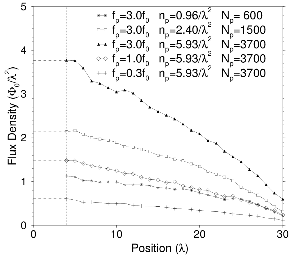
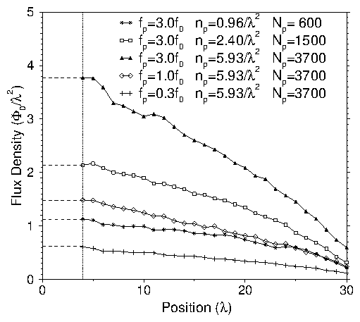
Figure 1: Magnetic flux density profiles B(x) for each sample studied. The profiles were obtained using B(x)=(24λ)⁻¹ ∫₀^24λ dy B(x,y). The area 0 < x < 4 λ, 0 < y < 24λ, to the left of the dotted line, is the unpinned region through which vortices enter the sample. This mimics the external field; the dashed line indicates the field strength in this region. The presence of bulk pinning in the sample (located in the region 4λ < x < 30 λ, 0 < y < 24λ) provides a barrier for flux entry and exit at the interface x=4λ. 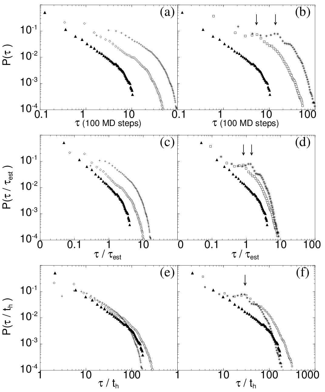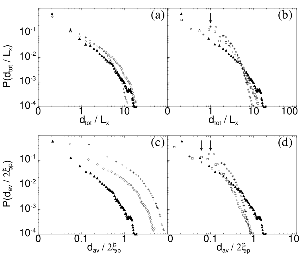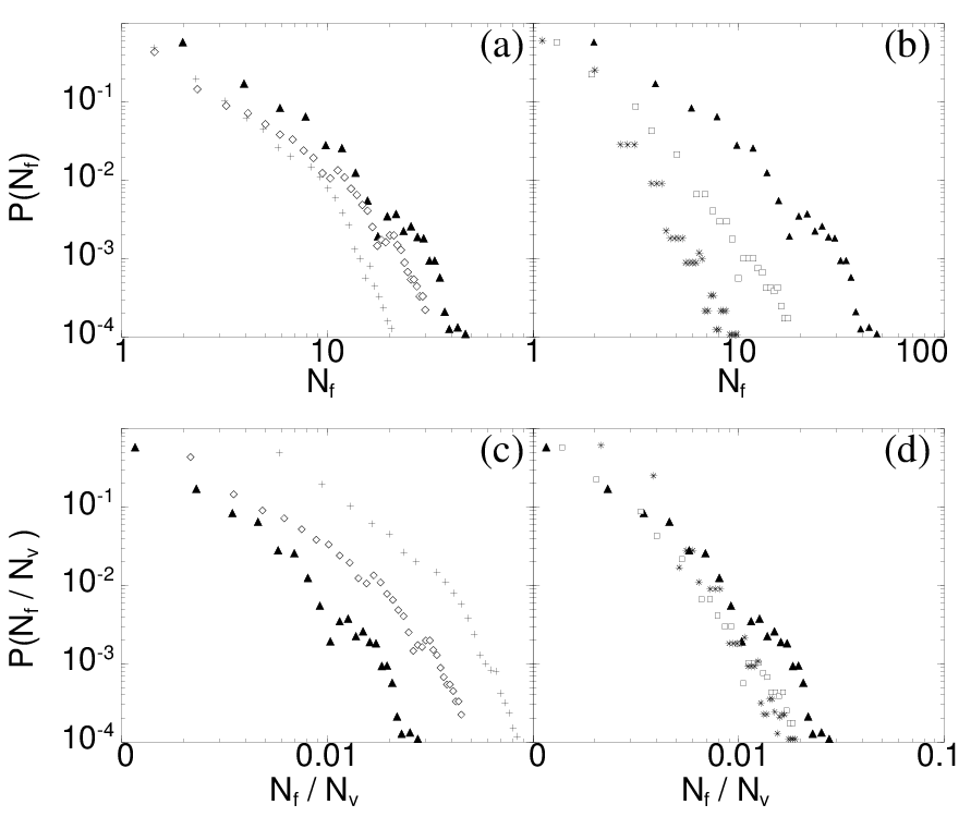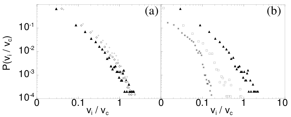The five profiles correspond to five samples with three different densities of pinning sites, n_p, and three different uniformly distributed pinning strengths, f_p. Starting from the top (very strong pinning) to the bottom, we have filled triangles: f_p^max=3.0 f₀, n_p=5.93/λ², N_p=3700, N_v ≈ 1700; open squares: f_p^max=3.0 f₀, n_p=2.40/λ², N_p=1500, N_v ≈ 1000; open diamonds: f_p^max=1.0 f₀, n_p=5.93/λ², N_p=3700, N_v ≈ 700; asterisks: f_p^max=3.0 f₀, n_p=0.96/λ², N_p=600, N_v ≈ 500; and plus signs: f_p^max=0.3 f₀, n_p=5.93/λ², N_p=3700, N_v ≈ 240. Note that the slope of B(x), i.e., J_c(x), is somewhat larger towards the right edge of the sample where the flux density is lower and the effective pinning is larger. The average slope is not altered by avalanches since the majority of the vortices in the sample do not move during an avalanche.

III. VORTEX AVALANCHES

The flux profile in the sample (see Fig. 1) is maintained in a quasi-magnetostatic state, with only a single vortex added to the left side of the sample every time the sample reaches mechanical equilibrium [23]. Although this resembles granular sandpile experiments that add a single grain at a time to the apex of the pile [1,2], there are very important differences between granular systems and our vortex system: the vortex interaction has a much longer range, incorporating the effects of up to 100 nearest neighbors; inertial effects are negligible in this highly overdamped system; and the disorder is quenched (i.e., pinning sites are fixed) and tunable (that is, the effective pinning strength can be varied with field).

Figure 2: Plot of the average vortex velocity v_av, shown in normal (a) and expanded (b) views. The box in (a) indicates the region expanded in (b). This quantity resembles voltage signals induced by moving vortices in actual experimental samples [11]. An additional vortex is added to the left edge of the sample only when v_av falls below the threshold (background) value of v_th=0.0006 f₀/η. Every period of avalanche activity can be clearly resolved. Certain velocity bursts composed of several closely spaced peaks in v_av correspond to single avalanches in which several vortex chains move consecutively in a manner resembling lightning strikes. In these avalanches with multiple peaks in v_av, the disturbance does not propagate through the sample at constant v_av in one pulse, but moves in repeated pulsing waves. This signal is from a sample containing 1700 vortices interacting with a high density of strong pinning sites: n_p=5.93/λ², f_p^max=3.0f₀.

To gauge the amount of vortex motion occurring in a sample at each MD time step, we use the average vortex velocity v_av, given by the sum of the magnitude of the velocity of each vortex v_i divided by the number of vortices in the sample N_v,

v_av=

N_v

N_v
∑
i=1

v_i .

(3)

We add a new vortex only when significant motion has stopped, as indicated when

v_av < v_th ,

(4)

where v_th is a low threshold value. The signal v_av is plotted in Fig. 2 for a sample with a high density of strong pinning sites and a threshold level v_th=0.0006 f₀/η. Each time a new vortex is added to the sample, a very small peak appears in v_av. Larger peaks are produced during the avalanches that are occasionally triggered by the addition of a vortex, with the largest peaks generated by a combination of either a few vortices moving rapidly or a large number of vortices moving slowly. Many avalanche events produce v_av signals that consist of several peaks clustered together, indicating that the avalanche disturbance does not propagate through the sample at constant v_av, but moves in repeated pulsing waves [25]. This burst-like behavior is a result of the combined effects of the vortex density gradient and the two-dimensional nature of the vortex motion.

Most avalanche disturbances start at the outer sample edge (left edge in the figures) where the vortex density is highest. When a vortex inside the sample is displaced from its pinning well due to a small increase in the external field, pinned vortices ahead of it prevent it from moving down the gradient. This is in contrast to granular sandpiles, where sand grains can move in the third dimension to avoid such blockages. A string of vortices is depinned in a domino-like effect, with each moving only far enough to depin the next vortex and then stopping. This pulsing motion continues until the forces on all vortices in the sample are once again below the threshold depinning force.

By adding only one vortex at a time, we probe the system in the limit of a zero current of incoming vortices. Large values of the current do not produce well-defined individual avalanches, so it is important that a given avalanche die away completely before adding the next vortex. Adding many vortices simultaneously, or at a very fast rate, can significantly modify the state of the system. The information we learn about a rapidly driven system tells us not about the original state but about the (possibly drastically) modified state. Use of an effectively infinitesimal perturbation allows us to avoid altering the nature of the original system while still gaining information about it, something that is important in other systems as well. For instance, in classical mechanics, a very small perturbation is applied to a particle to test the stability of its orbit. In electromagnetic systems, a small test charge is added to systems in order to probe their electrical screening or dielectric properties. In many-body physics, a very small electric or magnetic field is applied to systems to determine their diamagnetic response.

Voltage bursts and intermittency

The time-evolution of the velocity signal plotted in Fig. 2 resembles that observed for a variety of different physical systems in the so-called intermittent regime [26,27]. In particular, the general features of the velocity signal in Fig. 2 are similar to the fluid velocity at a point in the interior of the container in Rayleigh-Bénard convection experiments [28] in the intermittent regime. In the vortex and fluid cases, the somewhat regular velocity signals are intermittently interrupted by velocity "bursts" of finite duration which occur at seemingly random times. This section explores the conceptual analogies and differences between the velocity bursts produced by vortices moving in superconductors and the velocity bursts observed in intermittency. A quantitative and detailed comparison is beyond the scope of this section, and will be presented elsewhere.

Let us first summarize the intermittent transition to chaos [29]. More information can be found in Refs. [26,27]. Intermittency refers to a signal that alternates in an apparently random manner between long regular phases, known as laminar phases or intermissions, and relatively short irregular bursts, called chaotic bursts. The frequency of these bursts increases with an external parameter that we call ϵ here. Thus, intermittency provides a continuous route from regular, burst-free motion, for ϵ = 0, to chaotic motion, for large enough ϵ. For very small values of ϵ, there are long stretches of time, called laminar phases, during which the dynamics is regular, remaining very close to the burst-free ϵ = 0 fixed point.

Let us now consider a marginally stable Bean state. Take ϵ to be the rate at which vortices are added to the system (i.e., the driving rate). If ϵ = 0, the dynamical system of vortices is at a fixed point in both position and velocity spaces. In particular, its average velocity v_av is zero. In the language of nonlinear dynamics, the laminar phase now has an infinite duration and the motion is regular; that is, it is a fixed point of zero velocity.

When vortices are added to the system at a very small rate ϵ, such as one vortex added every 10⁵ MD steps, some vortices in the system rearrange their positions. In this case, the average vortex velocity remains very close to the v_av=0 laminar phase value, up to small oscillations produced by vortex rearrangements, In other words, if ϵ > 0 and very small, the velocity of the system remains quite near its v_av=0 fixed point (see, for instance, Fig. 50(b) of Ref. [26]). This dynamics near the fixed point, or "inside the laminar region", does not continue forever. Eventually, the system exhibits a burst; that is, v_av(t) suddenly increases to a larger value, producing a crest of apparently random shape, or a "chaotic burst". After a period of time that is typically short, this burst suddenly comes to an end, and the system is "reinjected into" the laminar region, exhibiting its usual dynamics near the fixed point. When vortices are added to the system at an increasingly large rate ϵ, the average vortex velocity displays more frequent bursts away from the v_av=0 fixed-point laminar phase value.

For chaotic systems in the intermittent regime, the length of time the system spends around its fixed point, and the length of time the system spends in the chaotic region, are both unpredictable. If the same computer run is repeated with initial conditions that vary slightly, the details of the dynamics will not be reproduced [26,27]. These and many other results have been obtained for chaotic systems in the intermittent regime. Analogous calculations have not been made for vortices in the Bean state. It would be interesting to calculate, among other things, the average time the system spends around its fixed point (i.e., in the laminar region) as a function of the driving rate ϵ. It is unclear at this point how these quantities compare for the vortex and standard nonlinear systems. To compute these quantities for vortices is far more complicated than for the usual systems. Fluid flow, modeled by the three Lorentz equations, and other intermittent systems (e.g., nonlinear RLC circuits) can be described effectively by few degrees of freedom. The problem of vortex avalanches requires solving very many degrees of freedom, which greatly complicates the calculations. These will be considered elsewhere.

IV. ANALYSIS OF THE SPATIOTEMPORAL EVOLUTION OF VORTEX AVALANCHES

The spatiotemporal propagation of avalanches through a sample are of great interest. The analysis presented below provides insight into which microscopic properties of a sample are most important in determining the nature of the resulting avalanches. Few experimental studies in any avalanche system are able to view individual avalanches. Experiments involving vortex avalanches so far have been able to resolve only a macroscopic result of the avalanche, such as flux leaving the sample, and have not been able to determine the path the vortices followed as they moved through the sample. Our simulations can easily image vortex avalanches, revealing how changing the microscopic pinning parameters affects the nature of the avalanches.

A. Spatial configurations of vortex avalanches

We first determine the path an avalanche follows through the sample by identifying the vortices involved in representative avalanche events. A vortex is considered an avalanche participant if it is depinned, indicated when its displacement d_i during the time interval between adding new vortices to the sample is greater than the pinning diameter 2 ξ_p,

d_i > 2 ξ_p .

(5)

This distinction is necessary since most vortices in the sample are displaced very slightly during an avalanche, but only a small number depin and are transported down the gradient. Because our simulation operates in the regime n_v < n_p, all vortices remain trapped at pinning sites when an avalanche is not occurring, except in the case of very low pin density when some vortices remain at interstitial sites created by the repulsion from surrounding vortices.

Figure 3: Snapshots of vortices participating in an avalanche event. Here, the initial positions of vortices that were depinned during the avalanche are represented by filled circles. Vortices that remained pinned are represented by crosses. Vortex motion is towards the right of the figure, and the entire 26 λ×24 λ sample is shown. Panel (a) is from a sample with n_p=5.93/λ² and f_p^max=3.0f₀; panels (b), (c), and (d) are from a sample with lower pinning density: n_p=2.40/λ² and f_p^max=3.0 f₀. (a) shows a large event. The stationary vortices in and around the flow path are more strongly pinned than the moving vortices and provide barriers to the flow. (b) is a typical chain-like event. Most events are this size or smaller. (c-d) show how a characteristic channel for motion can change slightly over time [e.g., from (c) to (d)]. Infrequent large events rearrange the vortices in (c) and alter the interstitial pinning caused by vortex-vortex interactions, resulting in the new channels shown in (d). In other words, the channels in (d) are produced by a vortex lattice rearrangement after the channels in (c) dominated the transport over several avalanches. Note the gradient in the vortex density, with a higher density on the left side of the figure.

A single avalanche event is depicted in each panel of Fig. 3. The entire sample is shown in each case, with the initial positions of vortices that were depinned during the avalanche marked with filled circles. The vortices that remained pinned are indicated with crosses. Rare large events, such as that illustrated in Fig. 3(a) for a densely pinned sample, involve a broad region of the sample. These events occur only after a considerable amount of strain has accumulated in the vortex lattice. In the most frequently occurring events, winding chains of vortices move from pinning site to pinning site, with each vortex moving into the site vacated by a vortex to its right, as in Fig. 3(b). The chains extend down the flux gradient in the x-direction, and are not perfectly straight but wind in the y-direction. The amount of winding increases as the pinning strength f_p decreases. The chains do not appear at the same location during every avalanche, and chain size may vary: in some events a chain spans the sample, while in others the chain contains only three or four vortices.

When the pinning density is high, moving vortex chains are equally likely to form anywhere in the sample. As the pinning density is lowered, however, the probability that the movement will occur in a certain well-defined channel at one location in the sample becomes very high. The position of this channel varies from sample to sample, but all samples with low pinning density contain such a channel. An example of a "preferred channel" is illustrated in Fig. 3(c,d). Here the vortices follow the same winding path during several consecutive avalanches. These meandering vortex channels display branching behavior or form small loops around stronger pinning sites. As a result of the low pinning density in the sample shown in Fig. 3(c,d), interstitial pinning is highly important. Interstitial pinning occurs when a vortex is held in place only by the repulsion from surrounding core-pinned vortices. Since the strength of the interstitial pinning is significantly weaker than that of the surrounding core pinning sites in a sample, as in Fig. 3(c,d), the resulting avalanches follow easy-flow paths composed almost entirely of interstitially pinned vortices. The occasional large events in such a sample rearrange the interstitial pinning landscape, leading to the formation of a new set of flow channels that will persist for a period of time until the next large event occurs. For example, the persistent flow channel of Fig. 3(c) was altered into the channel of Fig. 3(d) by a large event.

A small packet of flux never actually moves from one end of the sample to the other in a single avalanche, regardless of whether vortices move in fixed channels or in constantly changing paths. Instead, movement is transmitted from vortex to vortex, with an individual vortex rarely moving more than one to two pinning sites away from its former location during an avalanche. Thus, the disturbance crosses the sample, but a vortex does not, and the time span of a typical avalanche, τ, (measured below) is much shorter than the time required for a single vortex to traverse the sample.

B. Snapshots of the velocity field

The images analyzed above show that avalanche disturbances involve several possible types of moving bundles or chains of vortices, but give no information about the time scales for vortex motion. Thus, to examine the avalanche dynamics, we consider the velocities of individual vortices at several instants during an avalanche and present a series of snapshots of the vortex movements during a single avalanche. We find that avalanche disturbances propagate neither instantly nor at constant speed through the sample.

Figure 4: Consecutive snapshots of the vortex velocity field in a 25 λ×5 λ region of a 26λ×24λ sample with a high density of strong pinning sites, n_p=5.93/λ², f_p^max=3.0 f₀. Each moving vortex is indicated by an arrow whose length is scaled by the velocity of the vortex; the remaining vortices are indicated by small crosses. All vortices sit in pinning sites (not shown) when not in motion. A vortex is considered "moving" if it is depinned. The remaining vortices are not completely motionless, but shift very slightly inside the pinning sites. The disturbance propagates from the dense left edge of the sample to the relatively less dense right edge. The vortices in the rest of the sample (not shown) were not depinned. The time interval between snapshots is the typical time t_h required for a vortex to hop from one pinning site to another. The illustrated motion is typical of a medium-sized avalanche in this sample.

Figure 4 shows an avalanche moving through a portion of a sample with a high density of strong pinning sites. An arrow of a length proportional to the instantaneous vortex velocity marks the initial position of each moving vortex. The velocity of the vortices near the right edge of the sample is greater than that near the left edge due to the vortex density gradient. The uniform time interval separating each panel was chosen as t_h, the time required for a vortex to hop from one pinning site to the next, so that most vortices complete their motion within one panel of the figure. The disturbance in this avalanche propagates through the sample, with most of the vortices involved stopping exactly one pinning site to the right of their initial positions. Thus, the majority of the motion occurs inside the sample and cannot be detected by probing only vortices exiting the sample. Those vortices that do exit have initial positions within one to two lattice units from the sample edge, and we do not observe vortices moving many pinning sites to the right during a single avalanche in order to leave the sample. We therefore find that during the largest avalanches, when the greatest number of vortices exit the sample, all movement and flux exit occurs in a wide region of the sample. Fig. 3(a) shows an example of a wide avalanche.

The event pictured in Fig. 4 has a medium-length lifetime. Events with longer lifetimes often consist of more than one pulse of motion; that is, the average velocity v_av exhibits several spikes or oscillations during a single avalanche.

C. Cumulative pattern of vortex flow channels

The spatial configurations of the avalanches we observe are not strongly affected by the sample pinning parameters, with all samples producing vortex motion in winding chains that propagate through the sample during one or more pulses. The pinning parameters are important, however, when we consider whether chains moving in consecutive avalanches are concentrated in one area of the sample, or whether they are evenly distributed throughout the sample over time. By plotting the vortex trajectories with lines, and drawing these lines for an extended period of time covering many avalanches, we can identify the cumulative pattern of vortex flow channels for different pinning parameters. Heavily-traveled regions of the sample are easily distinguished by a concentration of trajectory lines. An examination of small regions of samples shows that the typical flow channel pattern varies with pinning density.

Figure 5: Continuous lines indicate the paths vortices follow through a portion of the sample over an extended period of time covering many avalanches. Vortices enter through the left edge and move towards the right edge. Dots represent vortices, and open circles represent pinning sites. An 8λ×8λ region of the 26λ×24λ sample is shown. (a) n_p=0.96/λ², f_p^max=3.0 f₀. (b) n_p=2.40/λ², f_p^max=3.0 f₀. (c) n_p=5.93/λ², f_p^max=3.0 f₀. (d) n_p=5.93/λ², f_p^max=0.3 f₀. Vortex motion in the sample with n_p=5.93/λ², f_p^max=1.0 f₀ resembles (c) and (d). In (a) and (b), strong pinning occasionally causes segments of the vortex path to run towards the top and bottom of the figure, transverse to the flux gradient. The presence or absence of easy-flow channels is strongly dependent on pin density. The channels present in (a) and (b) lead to avalanches with characteristic sizes N_a and lifetimes τ. Samples with higher pinning density do not have isolated easy-flow channels and produce very broad distributions of avalanche sizes. Because of the higher pinning strength, avalanches in (c) have higher typical vortex velocities v_i and shorter typical event lifetimes τ than those in (d), resulting in tighter, less wandering vortex paths.

As shown in Fig. 5(a-b), interstitial channels of easy flow for vortices develop in samples with a low density of strong pinning sites. The flow of flux lines in Fig. 5(a) involves only the much more mobile interstitial vortices moving plastically around their strongly pinned neighbors, indicated by the fact that the vortex trajectories form narrow paths that never intersect the pinning sites. Similar behavior has been directly observed recently by Matsuda et al. [16], where interstitial, chain-like avalanche flow was seen around a few strongly pinned vortices [30]. As the pin density is increased, pin-to-pin vortex motion becomes more important and the interstitial channels become less well defined [Fig 5(b)] until at the highest pin densities, n_p=5.93/λ², interstitial flow is no longer observed, and the vortices always move from pinning site to pinning site. This is illustrated in Fig. 5(c-d) for a high density of pins of two different strengths. Note the absence of distinct isolated flow channels.

D. Derivation of the criteria for the presence of interstitial vortex motion

In the limit of strong pinning, we expect interstitial vortex motion to occur whenever a vortex moving between two pinned vortices exerts a maximum force f^vv_midpoint on each pinned vortex that is less than the pinning force f_p. This occurs at the midpoint between the two pinned vortices. If this condition is not met, one of the pinned vortices will be depinned, and the interstitial vortex might be trapped by the vacated pinning site. Given the pinning density n_p of a sample, we can calculate the minimum pinning strength f^(p)_min required to allow interstitial motion. Assume that two vortices are pinned in adjacent wells separated by the average distance d_p=n_p^−1/2 between pinning sites. If an interstitial vortex passes directly between these two pinned vortices, it is a distance d_p/2 from each pinned vortex, and exerts a force on each equal to

f^vv_midpoint = f₀ K₁

⎛
⎝

d_p

2λ

⎞
⎠

(6)

For interstitial motion to occur, we require

f^(p)_min = f^vv_midpoint .

Thus,

f^(p)_min = f₀ K₁

⎛
⎝

d_p

2λ

⎞
⎠

f^(p)_min = f₀ K₁

⎛
⎜
⎝

2λ

√

n_p

⎞
⎟
⎠

(7)

For each of the pinning densities used in our simulation, we can determine the minimum pinning strength f^(p)_min that would permit interstitial motion. In samples with a high density of pinning sites, n_p=5.93/λ², as in Fig. 5(c,d), we find f^(p)_min = 4.7f₀. Since the actual pinning forces in these samples are f_p <~3.0f₀, we do not expect interstitial motion to occur, and the simulations confirm that only pin-to-pin motion occurs in these samples. Samples with a lower pinning density of n_p=2.40/λ², as in Fig. 5(b), have f^(p)_min = 2.8f₀. In this case, with f_p <~3.0f₀, occasional interstitial motion may occur near the strongest pins, and a small amount of interstitial motion is observed in the corresponding simulations. In samples with the lowest pinning density of n_p=0.96/λ², as in Fig. 5(a), f^(p)_min = 1.6f₀. This condition is easily met by a large portion of the pins, which have f_p <~3.0f₀, and exclusively interstitial vortex motion is expected and observed in the simulations.

V. STATISTICAL DISTRIBUTIONS CHARACTERIZING VORTEX AVALANCHES

The strikingly different behaviors of the vortex avalanches are quantified here by identifying the dependence of the distributions of several quantities on pinning parameters. These quantities include: τ, the avalanche lifetime; N_a, the number of vortices participating in the avalanche; N_f, the number of vortices exiting the sample during an event; d_tot, the total vortex displacement occurring in the avalanche; as well as d_i and v_i, the individual vortex displacements and velocities during an avalanche.

A. Avalanche lifetime

A frequently used characterization of an avalanche is its total lifetime, τ, or the interval of time during which the avalanche occurs. In our simulation, τ is equal to the interval between perturbations of the system by the addition of a new vortex. Recall that here, the Bean state is always driven in a quasimagnetostatic mode: a flux line is added, vortex positions in the sample shift and may produce an avalanche, and the next flux line is added only after the vortex lattice reaches mechanical equilibrium. We expect the avalanche lifetime to depend on both the pinning strength and the pinning density.

The pinning strength f_p influences avalanche lifetimes by determining the speed of vortex motion in the sample. We find a relationship between the pinning strength f_p and the speed v_i of an individual vortex by considering the behavior of a vortex at position r_i immediately after it is depinned from a well at position r_k^(p). If we assume that the vortex barely has enough energy to escape the well, the total force on the vortex just before it depins is close to zero:

f_i=f_i^vv + f_p

≈ 0 ,

(8)

where

f_p=| f_i^vp(|r_ik|=ξ_p) |

(9)

is the maximum pinning force at the edge of the parabolic well, ∧r_ik = r_ik/|r_ik| = (r_i − r_k^(p))/|r_i − r_k^(p)|, and r_ik is the distance between vortex i and the center of the kth parabolic well. Thus,

f_i^vv ≈ − f_p

(10)

The pinning force has an abrupt cutoff at the pinning radius ξ_p, so when the vortex moves off the pinning site, the vortex-pin force f_i^vp suddenly falls to zero while the long-range vortex-vortex force f_i^vv changes only negligibly. The resulting force on the vortex is

f_i=f_i^vv ≈ −f_p

(11)

Thus, the vortex velocity is

v_i=v_c=

|f_i|

≈

f_p

(12)

where v_c is a characteristic velocity associated with the pinning strength. Vortices in samples with stronger pinning move faster when depinned than vortices in samples with weaker pinning.

Figure 6: Distributions of avalanche lifetimes, τ. The leftmost panels (a,c,e) correspond to our highest density of pins, n_p=5.93/λ², and differing pinning strengths: filled triangles, f_p^max=3.0 f₀; open diamonds, f_p^max=1.0 f₀; plus signs, f_p^max=0.3 f₀. The right panels (b,d,f) correspond to samples with our strongest pins, f_p^max=3.0 f₀, and differing pinning densities: filled triangles, n_p=5.93/λ²; open squares, n_p=2.40/λ²; asterisks, n_p=0.96/λ². (c-d) Distributions scaled by the estimated lifetime, τ_est. Note the appearance of characteristic avalanche times indicated by arrows in (d) at τ/ τ_est ≈ 0.8 and τ/ τ_est ≈ 1.3. (e-f) Distributions scaled by the hopping time, t_h. In (e) the hopping time between pinning sites is t_h=6, 18, and 57 MD steps, respectively. Also in (e), notice the power law behavior P(τ/t_h) ∼ (τ/t_h)^−1.4 for small τ/t_h over two decades for the sample with a high density of strong pins (filled triangles). In (f) the hopping time between pinning sites is t_h=6, 17, and 53 MD steps, respectively. The arrow in (f) at τ/t_h ≈ 30 indicates a local maxima in P(τ/t_h) for the two samples with lower density of pins. Panel (g) schematically indicates the notation used in the figures of this work.

In order to directly relate vortex velocities to avalanche lifetimes, we consider the distance an individual vortex moves during an avalanche event. A vortex normally hops from one pinning site to an adjacent site during the event. The distance it travels is simply d_p, the average distance between pinning sites,

d_p=

√

n_p

(13)

If we define a "string" avalanche as an event during which each vortex in a chain extending the length of the sample hops from one site to the next, we can estimate a "string" lifetime. First, we designate the time that a vortex with just enough energy to depin spends moving between pins as the hopping time, t_h.

t_h=

d_p

v_c

≈

f_p

√

n_p

(14)

For example, in PbIn, η ∼ 3.3 ×10⁻⁸ G²-s [32], so using f_p = 3.0 f₀, n_p = 5.93/λ², and λ ∼ 65 nm gives t_h ∼ 15 fs. Next, we estimate N_h, the number of vortices that must hop in order for the avalanche to span the sample:

N_h=L_x √n_v ,

(15)

where L_x is the sample length. If we assume that the vortices hop one at a time in sequence, we obtain an estimate of the "string" avalanche lifetime,

τ_est=t_h N_h ≈

ηL_x

√

n_v

f_p

√

n_p

(16)

For instance, using the value of t_h for PbIn given above and taking the vortex density to be n_v = 2.5/λ² gives a lifetime of τ_est ∼ 0.6 ps. The relationship between τ_est and f_p and n_p is not simple because the vortex density n_v=n_v(H,f_p,n_p). For a given field strength, however, it is clear that avalanche lifetimes decrease as pinning strength or density is increased. This is confirmed in the plot of the distribution P(τ) in Fig. 6(a-b), where we see that samples with strong dense pinning have significantly shorter avalanche lifetimes than samples with weaker pinning [Fig. 6(a)] or samples with lower pinning density in which interstitial pinning is important [Fig. 6(b)]. All histograms have been smoothed as described in Ref. [33].

In order to determine what fraction of the avalanches have lifetimes on the order of the estimated "string" lifetime τ_est, we scale the avalanche lifetimes by τ_est, and plot P(τ/τ_est) in Fig. 6(c-d). For the dense strong pinning case of Fig. 6(c), most avalanche lifetimes are shorter than the estimated lifetime τ_est (τ/τ_est < 1) as a result of two factors. First, several vortices hop simultaneously, as in Fig. 4, rather than hopping one after the other, as assumed in our estimate. Second, although Fig. 3 illustrated several system-spanning avalanches, many events do not involve enough vortices to span the entire sample but contain only a short chain of vortices moving a short distance. The majority of avalanches in samples with strong pinning, f_p^max=3.0f₀, contain less than ten vortices traveling in short chains that originate in regions of high vortex density but do not extend into areas with lower vortex density.

As the pinning force is lowered, the chains of moving vortices become longer on average, leading to an increase in the average value of τ/τ_est. Only samples with a reduced pinning density, shown in Fig. 6(d), produce frequent "string" avalanches. In these samples, nearly all avalanches occur in a single easy-flow channel that spans the sample, as in Fig. 5(a), or in two main channels as in Fig. 5(b). As a result, we observe an increased likelihood for the "string" avalanche in the form of an increase in the distribution function near τ/τ_est ≈ 1. This increase is most pronounced for the lowest pin density, n_p=0.96/λ² [Fig. 6(d)], where the channel is most strongly established. Since the channels in such samples wind significantly in crossing the sample, the number of vortices moving during the avalanche is greater than the estimated value N_h, and the observed increase in P(τ/τ_est) for n_p=0.96/λ² falls at τ/τ_est ≈ 1.3, rather than at τ/τ_est ≈ 1.

Figures 6(e-f) show the scaling of the avalanche lifetimes by the hopping time t_h. In this case, the distributions P(τ/t_h) for high pinning density (n_p=5.93/λ²), in Fig. 6(e), collapse and can be approximated for small τ by the form

⎛
⎝

t_h

⎞
⎠

∼

⎛
⎝

t_h

⎞
⎠

−γ

where

γ ∼ 1.4 .

Distributions generated by samples with lower pinning densities, in Fig. 6(f), do not scale and cannot be represented by the same form. This indicates the importance of the nature of avalanche propagation. For samples with a high density of pins, pin-to-pin vortex motion occurs throughout the sample, with all regions of the sample participating in an avalanche at some time. Once the pinning density decreases, however, interstitially pinned vortices appear and dominate avalanche transport. The vortices always follow the same paths, visiting as many interstitial sites as possible when moving through the sample, and introducing a characteristic avalanche lifetime.

B. Number of vortices in each avalanche

Figure 7: Distributions of the number of vortices, N_a, moving during an avalanche event. The left panels (a,c,e) correspond to samples with a high pin density, n_p=5.93/λ², and differing pinning strengths: filled triangles, f_p^max=3.0 f₀; open diamonds, f_p^max=1.0 f₀; plus signs, f_p^max=0.3 f₀. The right panels (b,d,f) correspond to samples with strong pins, f_p^max=3.0 f₀, and differing pinning densities: filled triangles, n_p=5.93/λ²; open squares, n_p=2.40/λ²; asterisks, n_p=0.96/λ². (c-d) Distributions scaled by the average number of vortices, N_h, that must hop for the avalanche to cross the sample. In (d), note the appearance of a characteristic value in the latter two samples at N_a / N_h ∼ 1. (e-f) Distributions scaled by the average number, N_v, of vortices in the sample. For samples with a large density of strong pins, the leftmost curve in (e) indicates that most avalanches involve only a tiny fraction of the vortices, resulting in plastic transport that occurs in brief, choppy bursts.

Avalanches can be characterized according to the number of vortices displaced during the event. This quantity can be directly observed through computer simulations, but at present must be inferred from experiments [11]. We define the number of vortices, N_a, that were actively moving participants in each avalanche as the number of vortices that were depinned. Figure 7(a-b) presents the corresponding distribution P(N_a). For high pinning density, as in Fig. 7(a), we can approximate the distribution for small N_a as

P(N_a) ∼ N_a^−β .

We find that β decreases as the pinning strength decreases:

β ∼

⎧
⎪
⎨
⎪
⎩

1.4 ,

f_p^max=3.0f₀

1.0 ,

f_p^max=1.0f₀

0.9 ,

f_p^max=0.3f₀

Smaller values of β indicate a relative increase in the frequency of large avalanches compared to small ones. The trend in β might appear counterintuitive since the smaller flux gradient present in systems with lower pinning strength f_p produces less energetic avalanches that might be expected to have small values of N_a. It is, however, the width of the avalanche disturbance rather than the magnitude of the flux gradient that is important in determining N_a. In samples with strong pinning, energetic avalanches occur, but avalanche width is suppressed since strongly pinned vortices on either side of the moving chain are not depinned during the short interval when vortices are moving very rapidly down the steep vortex density gradient. As the pinning weakens, avalanches become wider when weakly pinned vortices adjacent to a slowly moving chain depin and join the motion down the shallow gradient, resulting in more events with relatively large values of N_a.

Vortices flow only in certain channels when n_p is low, leading to the appearance of a characteristic value in P(N_a) [arrow in Fig. 7(b)] and making it impossible to describe P(N_a) by a power law form over the entire range of observed N_a values. The formation of avalanches with large values of N_a is impeded in such cases because all available interstitially pinned vortices are already participating in the channel, and the neighboring strongly pinned vortices cannot be depinned.

The arrow in Fig. 7(b) indicates a value of N_a corresponding to the number of vortices in the channels N_channel. Since the channels span the sample, we expect N_channel to be close to the number of vortices N_h that must hop to cross the sample in a straight chain, where N_h=L_x √n_v. To verify this, we plot the scaled quantity P(N_a/N_h) in Fig. 7(c-d). We find in Fig. 7(d) that samples with low pin density n_p, in which interstitial pinning is important, have N_channel ∼ N_h, as is expected if all moving vortices form a single chain across the sample. Specifically, increases in P(N_a/N_h) fall at N_a/N_h ≈ 1 for n_p=2.40/λ² and N_a/N_h ≈ 1.1 for n_p=0.96/λ². The winding of the channels in samples with n_p=0.96λ² causes the value of N_a corresponding to channel motion to be slightly larger than N_h. For samples with high pinning density, Fig. 7(c) indicates that the most linear part of P(N_a/N_h) is produced for N_a <~N_h, or for events that did not cross the entire sample. Broad avalanches are more than one vortex chain wide and have N_a/N_h > 3. These avalanches are more common in samples with smaller f_p, as indicated by the rightmost curve in Fig. 7(c), where samples with weak pinning provide the largest avalanches for a fixed probability density P(N_a/N_h).

To determine how effectively avalanches transport vortices across the sample, we scale N_a by the total number of vortices N_v present in the sample, and plot the result in Fig. 7(e-f). Only a tiny fraction of the vortices participate in a typical event when pinning is strong and dense, as indicated by the leftmost curve in Fig. 7(e). The avalanches in this sample are also very short lived, as already shown in Fig. 6(a), so this sample is best characterized by plastic transport that occurs in brief, choppy bursts. On the other hand, for a high density of weak pinning sites, we find that it is possible for a significant portion of the vortices in the sample to collectively move in an avalanche, as in the rightmost curve of Fig. 7(e). Vortex motion in these long-lived avalanches is less plastic, with small adjacent portions of the vortex lattice gradually sliding forward at different times. The samples with low pin density, shown in Fig. 7(f), have their transport dominated by the single easy-flow channel that develops. We find that the fraction of vortices contained in this channel increases as pinning density decreases since the interstitial channel winds to a greater degree in the sample with fewer pins and involves a correspondingly larger number of vortices.

C. Total vortex displacement

Figure 8: (a-b) Distributions of the total distance, d_tot, moved by all vortices in the sample scaled by the width of the sample, L_x. (c-d) Distributions of the average distance, d_av, traveled by a vortex during an avalanche event scaled by the pin diameter, 2ξ_p. The left panels (a,c) refer to samples with high pin density, n_p=5.93/λ², and differing pinning strengths: filled triangles, f_p^max=3.0 f₀; open diamonds, f_p^max=1.0 f₀; plus signs, f_p^max=0.3 f₀. The right panels (b,d) refer to samples with strong pinning, f_p^max=3.0 f₀ , and differing pinning densities: filled triangles, n_p=5.93/λ²; open squares, n_p=2.40/λ²; asterisks, n_p=0.96/λ².

Another measure of avalanche size, uniquely available through simulation, is the total displacement d_tot of all vortices in the sample during the event,

d_tot=

N_v
∑
i=1

d_i ,

(17)

where d_i is the displacement of each vortex. In order to find the probability of an avalanche that spans the sample length with d_tot >~L_x, we plot P(d_tot/L_x) in Fig. 8(a-b). Occasionally we observe avalanches with the surprisingly large d_tot/L_x ∼ 10. These large values reflect the cumulative effect of vortices that experience very small displacements inside the parabolic pinning sites rather than moving to a new pinning site. For instance, if 800 vortices each move a distance d_i ∼ ξ_p/10=0.015 λ, the total displacement recorded would be 12 λ. Such very small vortex displacements play a very important role in transmitting stress throughout the vortex lattice. Figure 8(a) indicates that P(d_tot/L_x) is very robust against variations in pinning strength. Excluding large values of d_tot/L_x, the distributions can be approximated by the form

⎛
⎝

d_tot

L_x

⎞
⎠

∼

⎛
⎝

d_tot

L_x

⎞
⎠

−δ

We find that δ decreases as the pinning strength decreases:

δ ∼

⎧
⎪
⎨
⎪
⎩

1.7 ,

f_p^max=3.0f₀

1.2 ,

f_p^max=1.0f₀

1.1 ,

f_p^max=0.3f₀

Figure 8(b) indicates that P(d_tot/L_x) is weakly dependent on n_p. The effect of the channels appears as an enhancement of the distribution near d_tot/L_x=1, marked by an arrow in Fig. 8(b).

We can compare the relative amount of vortex transport in different samples by considering the average distance d_av moved by a vortex during an avalanche,

d_av=

N_v

N_v
∑
i=1

d_i =

d_tot

N_v

(18)

Since most vortices do not become depinned, we plot P(d_av/2ξ_p), where 2ξ_p is the diameter of the pinning trap. The plot of P(d_av/2ξ_p) in Fig. 8(c) shows that as the pinning strength f_p is reduced, d_av/2ξ_p increases, indicating that individual vortices are likely to travel further during an avalanche. This occurs both because a large fraction of vortices in samples with weak pinning participate in the avalanche, as demonstrated in Fig. 7(e), and because the average spacing between vortices increases since vortex density decreases with decreasing pinning strength. In Fig. 8(d), we find that reducing the pinning density n_p can either increase or decrease d_av. As n_p decreases, the strength of the interstitial pinning sites decreases, allowing individual vortices to travel further. Not as many vortices are moving, however, since the motion is restricted to well defined channels. These two competing effects enhance P(d_av) at small values of d_av, but reduce it at large values.

Figure 9: (a-b) Distributions of the distance, d_i, traveled by individual vortices during all the avalanche events. Characteristic displacements d_h are marked with arrows. (c-d) Distributions scaled by the inter-pin distance, d_p. Only vortices that moved more than 1.0 d_p were directly participating in the avalanche. The rest were shifting very slightly in pinning wells and transmitting stress through the lattice. (e-f) Distributions P(d_i/d_p) for only those vortices that traveled a distance d_i < d_p, i.e., vortices that were not depinned. (g-h) Distributions P(d_i/d_p) for only those vortices that traveled a distance d_i > d_p, i.e., vortices that were depinned. The left panels (a,c,e,g) correspond to samples with a high density of pins, n_p=5.93/λ², and differing pinning strengths: solid line, f_p^max=3.0 f₀; dashed line, f_p^max=1.0 f₀; heavy solid line, f_p^max=0.3 f₀. The right panels (b,d,f,h) correspond to samples with strong pinning, f_p^max=3.0 f₀, and differing pinning densities: solid line, n_p=5.93/λ²; dot-dashed line, n_p=2.40/λ²; dotted line, n_p=0.96/λ².

D. Individual vortex displacements

The microscopic information available in our simulation permits us to calculate individual vortex displacements. In Fig. 9 we plot P(d_i), where d_i is the distance a single vortex is displaced in an avalanche. In every distribution, we find that vortex motion can be described in terms of a characteristic size d_h, indicated by arrows in the figure. This size roughly corresponds to the average distance between pinning sites d_p,

d_h ≈ d_p =

√n_p

(19)

and appears because vortices participating in an avalanche typically hop from one pinning site to an adjacent pinning site. Thus, in Fig. 9(a), d_h falls at the same value for three samples with equal pinning density n_p, while in Fig. 9(b), d_h increases as n_p decreases. The vortices in the sample can thus be divided into three categories: those that did not leave a pinning site, d_i < 2ξ_p < d_h, those that hopped from one pinning site to another, d_i ∼ d_h, and those that hopped more than one pinning site, d_i > d_h.

We first consider those vortices that hopped one pinning site. If we scale the distributions by the inter-pin distance d_p, as in Fig. 9(c-d), we find that the characteristic distances in P(d_i/d_p) fall at d_i/d_p ∼ 1 (marked with an arrow), with a second smaller increase at d_i/d_p ∼ 2 occurring in samples where vortices occasionally hopped two pinning sites.

Next we examine the motion of vortices shifting very slightly inside pinning wells. In Fig. 9(e-f), we focus on vortices that did not leave a pinning site, d_i < d_p, and present P(d_i/d_p). We find that, for small values of d_i/d_p, these distributions can be described by the form

⎛
⎝

d_i

d_p

⎞
⎠

∼

⎛
⎝

d_i

d_p

⎞
⎠

−ρ

where: ρ ≈ 1.4 for n_p=5.93/λ² and f_p^max=3.0f₀; ρ ≈ 1.4 for n_p=5.93/λ² and f_p^max=1.0f₀; ρ ≈ 1.4 for n_p=2.40/λ² and f_p^max=3.0f₀; ρ ≈ 1.2 for n_p=0.96/λ² and f_p^max=3.0f₀; and ρ ≈ 0.9 for n_p=5.93/λ² and f_p^max=0.3f₀. The two samples with smaller values of ρ also have the lowest critical currents J_c, as determined from the slope of the flux profiles in Fig. 1.

A simple two-dimensional argument shows that ρ is expected to be similar (and close to one) for all samples, since only vortices that experience extremely small displacements in pinning sites affect the value of ρ. If we add an additional vortex to an already existing arrangement of vortices, the repulsive force, f_extra, from this vortex will cause each nearby vortex to move a very small distance u_i in its pinning well in order to reach a new equilibrium position. Neglecting higher order effects, we find that the very small displacement u_i of the ith vortex is determined by the distance from the added vortex and by the form of the force f_extra. We take the distance from the perturbing vortex to be r, and assume that the additional force is applied during a time δt. The vortex-vortex interaction force gives

f_extra=

Φ₀²

8π²λ³

K₁

⎛
⎝

⎞
⎠

(20)

If we consider the limit of small r, r << λ, we can use the asymptotic form of the Bessel function to write

f_extra ≈

Φ₀²

8π²λ³

(21)

We have (for δu < ξ_p << λ)

δu(r) =

f_extra

δt ≈

δt

Φ₀²

8π²λ³

(22)

To obtain a distribution, we find the number of vortices N(r) located a radius r from the perturbing vortex. Due to the cylindrical symmetry, this can be written simply as

δN(r)=2πr n_v δr ,

(23)

where δr is an infinitesimal displacement. We want an expression for the slope of our distributions,

ρ = −

d(ln(δu))

lnδN .

(24)

Thus, we write:

lnδN(r)=ln(2 πn_v δr) + lnr

(25)

d lnδN(r)

(26)

lnδu(r) ≈ ln

⎛
⎝

Φ₀²δt

8π²λ²η

⎞
⎠

− lnr

(27)

d lnδu

≈ −

(28)

Therefore, we find

−ρ =

d lnδN

d lnδu

≈

⎛
⎝

⎞
⎠

⎛
⎝

−

⎞
⎠

−1

=−1 .

(29)

For small displacements (δu < ξ_p << λ), this predicts ρ ∼ 1, in general agreement with our observed values (ρ ≈ 0.9 − 1.4).

The argument presented above is independent of the shape of the pinning potential, and assumes that the vortex density n_v is constant throughout the sample. The presence of the Bean critical state makes this assumption inaccurate. It can, however, be shown that including the critical state does not significantly affect the expected value for the slope. We describe the field in the sample according to the Bean model,

B=H_ext −

2πJ_cr

(30)

where H_ext is the externally applied field. The field can also be written as

B=n_vΦ₀ .

(31)

Thus,

n_v(r)=

H_ext − 2πJ_cr/c

Φ₀

(32)

The number of vortices located at a distance r becomes

δN(r)=2πr

(H_ext − 2πJ_cr/c)

Φ₀

δr .

(33)

We then have

lnδN(r)=ln

⎛
⎝

2πδr

Φ₀

⎞
⎠

+ lnr + ln(H_ext − 2πJ_cr/c)

(34)

d lnδN(r)

−2πJ_c/c

H_ext − 2πJ_cr/c

(35)

The external field H_ext can be written in terms of the critical current J_c and the distance the field has penetrated into the sample, r^*:

H_ext=

2πJ_c r^*

(36)

We obtain

d lnδN

d lnδu

≈ −1 −

−r

r^* − r

= −1 −

1−(r^*/r)

(37)

We have r^* >> r, since the field has penetrated the entire sample length L_x >> λ. We therefore write

d lnδN

d lnδu

≈ −1 −

⎛
⎝

r^*

⎞
⎠

1 − (r/r^*)

≈ −1 −

r^*

(38)

Thus, including the Bean gradient introduces only a negligible correcting term r/r^* to the expected slope, since r/r^* << 1.

It is interesting to consider what slope value would be obtained if the vortex-vortex interaction were that found in a thin film, rather than the form for a thick slab of material used above. In this case, the additional force from a vortex is

f_extra ∼

r²

(39)

giving

δu(r) ∼

ηr²

δt

(40)

lnδu(r) ∼ ln

δt

−2 lnr

(41)

d lnδu

∼ −

(42)

d lnδN

d lnδu

∼

⎛
⎝

⎞
⎠

⎛
⎝

−

⎞
⎠

−1

=−

(43)

Thus, the distribution of individual displacements in a thin film should differ from that produced by a slab of material (ρ ∼ 0.5 versus ρ ∼ 1).

In Fig. 9(g-h), we focus on the displacements of vortices that were actively participating in avalanches, and plot P(d_i/d_p) for vortices with d_i > d_p. We find that decreasing the pinning strength leads to a very slight overall increase in the distance traveled by a moving vortex, as indicated by the slightly higher likelihoods for moving larger distances in Fig. 9(g). This is a result of the fact that, in general, avalanche disturbances are larger and longer lived in these samples, allowing individual vortices the opportunity to travel two or more pinning sites in an avalanche. Decreasing the pinning density, as in Fig. 9(h), also affects the likelihood that a vortex will move a certain distance.

E. Vortices leaving the sample

Figure 10: (a-b) Distributions of the number N_f of vortices falling off the edge of the sample. (c-d) Distributions scaled by the average total number N_v of vortices in the sample. The left panels (a,c) correspond to samples with a high density of pins, n_p=5.93/λ², and differing pinning strengths: filled triangles, f_p^max=3.0 f₀; open diamonds, f_p^max=1.0 f₀; plus signs, f_p^max=0.3 f₀. When N_f is not very large, the slope of the curve in each case is roughly −2.4. The right panels (b,d) correspond to samples with strong pinning, f_p^max=3.0 f₀, and differing pinning densities: triangles, n_p=5.93/λ²; squares, n_p=2.40/λ²; asterisks, n_p=0.96/λ². For small values of N_f, the slope of the curves in (b) is roughly −2.4, −3.4, and −4.4, respectively.

The number of vortices N_f that exit the sample during an event can be directly compared with values obtained in experiments, both in vortex systems [11,12,13] and in sandpiles [1,2,3]. In Fig. 10(a-b) we plot P(N_f). Events with N_f=0 are not shown. The relatively small size of our sample resulted in a smaller data set for this quantity than for all other quantities considered in this paper. If we approximate the distributions for small N_f by the form

P(N_f) ∼ N_f^−α ,

we find that all samples with high pinning density have

α ∼ 2.4 .

As the pinning density n_p is decreased for constant f_p, α increases, with α ∼ 3.4 for n_p=2.40/λ² and α ∼ 4.4 for n_p=0.96/λ². A larger α indicates a relatively smaller likelihood for the occurrence of events with large N_f.

When we examine the region from which vortices exit the sample, we find that flux can exit from any location in samples with high pin density, as seen from the relatively uniform coverage of trails along the right (outer) edge of Fig. 5(c) and Fig. 5(d). Even after one location has been depleted by a large avalanche, other areas along the sample edge still contain enough vortices to remain active in large and small events while the depleted regions refill. As the pinning density is decreased and interstitial channels develop, avalanche paths become highly constrained and flux exits in only a few locations that have difficulty building up enough stress to permit events with large N_f to occur. For example, with the reduced number of flux paths in Fig. 5(b), events with large N_f are rare, and thus α is large: α ∼ 3.4. Fig. 5(a) illustrates a small region of the extreme case of a sample with only one exit channel, for which n_p=0.96/λ² and α has the larger value α ∼ 4.4. Large values of N_f occur only when this single channel is filled by vortices under high stress. Since all smaller events happen through this same channel, however, stress in the channel is relieved by small events before it can build to a high level. Thus, the likelihood that the channel will produce a very large N_f is extremely small. As expected, the cut-off of P(N_f) for this sample falls at a much lower N_f than that of the other samples, as seen in the leftmost curve in Fig. 10(b).

Strong pinning effectively confines the avalanche disturbance to a narrow channel and prevents movement from spreading throughout the sample. Weak pinning permits collective motion in larger regions of the sample. These effects are more pronounced for samples with a lower density of pinning sites. This is highlighted by a comparison of how effectively individual avalanches remove vortices from different samples. In Fig. 10(c-d), we scale N_f by the number of vortices in the sample N_v. Most vortices in a sample with strong pinning cannot exit; those that do exit move in isolated chains. As the pinning strength is weakened, however, a greater percentage of the vortices are able to exit in events that consist of the collective motion of several adjacent chains. This is illustrated by the rightmost curves in Fig. 10(c).

F. Individual vortex velocities

Figure 11: Distributions of the individual velocities, v_i, of vortices in a thin strip of the sample, scaled by the characteristic velocity v_c. The left panel (a) corresponds to samples with a high pinning density, n_p=5.93/λ², and differing pinning strengths: filled triangles, f_p^max=3.0 f₀; open diamonds, f_p^max=1.0 f₀; plus signs, f_p^max=0.3 f₀. The right panel (b) corresponds to samples with strong pinning, f_p^max=3.0 f₀, and differing pinning densities: triangles, n_p=5.93/λ²; squares, n_p=2.40/λ²; asterisks, n_p=0.96/λ².

Due to the presence of a non-uniform magnetic flux gradient that is not of the ideal Bean form, the velocity of an average vortex is a function of position (see Fig. 1). Therefore, to construct a distribution of individual vortex velocities v_i that is not affected by the gradient, we select a narrow region of the sample where the gradient is essentially constant and find P(v_i) for vortices in this region. The individual velocities v_i are then scaled by the characteristic velocity v_c, given by

v_c=

d_p

t_h

≈

f_p

(44)

where d_p is the average distance between pinning sites, and t_h is the average hopping time, t_h=ηd_p/f_p. Figure 11 presents the resulting distributions P(v_i/v_c). For a high density of pinning [Fig. 11(a)], we find that pinning strength changes v_c but does not affect the form of P(v_i/v_c). Note that vortices moving at speeds less than v_c do not have sufficient energy to escape from a pinning site and are merely experiencing very small displacements inside their respective pinning wells. The similar form of P(v_i/v_c) is then explained by the fact that all of the wells are parabolic. For the lowest velocities, we can approximate P(v_i/v_c) with

⎛
⎝

v_i

v_c

⎞
⎠

∼

⎛
⎝

v_i

v_c

⎞
⎠

−σ

where

σ ∼ 2 .

Different densities of pinning wells alter the form of P(v_i/v_c), as can be seen from Fig. 11(b). As the pinning density decreases, some vortices experience small displacements in interstitial wells while others remain in parabolic traps. The combined effect changes the overall distribution.

If, instead of considering the distribution of individual velocities, we construct the power spectrum of the velocity signal v_av, we find that all of the samples with a high pinning density produce broad power spectra S(f) of the form S(f) ∼ f^−ν, where 1.5 < ν < 2.0. Samples with lower pinning density do not produce spectra of this form. The noise power spectra will be discussed further elsewhere [34].

VI. RECENT EXPERIMENTS ON VORTEX PLASTIC FLOW AND AVALANCHES

In several experiments, the nature of the vortex movement has been inferred indirectly by using, for instance, voltage signals, resulting in several plausible scenarios of vortex motion including cylindrical bundles [17], clump-like bundles [32,35], or elongated bundles [36]. Due to the presence of a field gradient in the sample, we find that all collectively moving groups of vortices are arranged in one or more long, narrow moving chains rather than clumped or cylindrical bundles. The existence of quasi-one-dimensional vortex channels is suggested in Refs. [32,37], where vortex motion is assumed to occur in straight paths that cross the sample. The chain-like channels that we observe resemble these suggestions, except that in our simulation the vortex paths often wind through the sample rather than following the shortest path down the gradient. In addition, our simulation indicates that the velocity of the moving vortices during a single avalanche is not constant but is pulse-like, that is, with oscillations in the average velocity v_av during the vortex avalanche.

Quantity	f_p^max = 0.3f₀	f_p^max = 1.0f₀	f_p^max = 3.0f₀	Ref. [11]	Ref. [13]
τ/t_h	γ ∼ 1.4	γ ∼ 1.4	γ ∼ 1.4	-	-
N_a	β ∼ 0.9	β ∼ 1.0	β ∼ 1.4	-	-
d_tot/L_x	δ ∼ 1.1	δ ∼ 1.2	δ ∼ 1.7	-	-
d_i/d_p	ρ ∼ 0.9	ρ ∼ 1.2	ρ ∼ 1.4	-	-
v_i/v_c	σ ∼ 2.0	σ ∼ 2.0	σ ∼ 2.0	-	-
N_f	α ∼ 2.4	α ∼ 2.4	α ∼ 2.4	α ∼ 1.4 to 2.2	α ∼ 1.7 to 2.2

Table 1: Best-fit slopes of the most linear region of distributions of several quantities. The form of the distributions in each case were: P(τ/t_h) ∼ (τ/t_h)^−γ, P(N_a) ∼ N_a^−β, P(d_tot/L_x) ∼ (d_tot/L_x)^−δ, P(d_i/d_p) ∼ (d_i/d_p)^−ρ, P(v_i/v_c) ∼ (v_i/v_c)^−σ, P(N_f) ∼ N_f^−α. Notice that a multiplicative factor in the independent variable does not alter the slope. Thus, τ and τ/t_h produce distributions with the same slope. The samples listed here had a high density n_p = 5.93/λ² of pinning sites. Samples with f_p^max = 3.0 f₀ and lower densities n_p of pins did not produce power law distributions.

In the experiment by Field et al. [11], flux lines exiting a superconducting tube were detected with a coil. Our average velocity signals, plotted in Fig. 2, strongly resemble the resulting voltage signals in Fig. 1 of Ref. [11]. Both simulation and experiment find distributions of avalanche sizes N_f that can be approximated by power laws with a range of exponents. The experiment in Ref. [11] finds α ∼ 1.4 to 2.2, while we find α ∼ 2.4 to 4.4 using a variety of different samples. The behavior of the experimental sample therefore resembles our simulations with a very high density of pinning sites, n_p=5.93/λ², and no characteristic channels. This is reasonable since the density of pinning in the experimental sample is very high. The pinning centers are grain boundaries with spacings randomly distributed between about 30 and 50 nm, while λ is on the order of 400 nm, leading to a pinning density of n_p ∼ 100/λ². Thus, this sample has a higher pin density than our most densely pinned case, and it is therefore reasonable to expect the experimental exponents to be less than 2.4 based on the general trend of our results.

Zieve et al. [12] observed avalanches at higher field strengths, where the pinning forces are expected to be reduced, and interpret their results to mean that the high-field regime produces large-scale, plastic rearrangements of the vortices, whereas the low-field regime generates elastic rearrangements. It is possible that there were undetectable steps in the hysteresis loops they obtained in the low-field regime since the smallest flux jumps resolved by their apparatus were on the order of 0.1 kOe. If their sample contained either characteristic channels for flux flow or high strength pinning, only a small fraction of the flux inside the sample would be transported through narrow exit regions at these low fields. As the field density increased, their sample would cross into the regime of weak dense pinning. In this case, as shown by our simulations, the sample can effectively transport much more flux, producing larger flux steps that can be resolved by the experiment.

Finally, we consider very recent work by Nowak et al. [13], who obtain different types of avalanche distributions as a function of temperature. At higher temperatures, they find a broad distribution for the amount of flux exiting the sample in each event,

P(N_f) ∼ N_f^−α ,

with α ranging from 1.7 to 2.2, in agreement with both Ref. [11] and our results. At the lowest temperatures, characteristic avalanche sizes appear in the form of events involving a large number of vortices that may be system-spanning. These changes have been discussed in terms of thermal instabilities in the material [13], but they can also be considered from the standpoint of the presence or absence of channels for vortex motion. As we have seen in our simulations, channels are most likely to form when the vortices are able to move interstitially. This is expected to happen whenever the pinning force exceeds the minimum pinning strength f^(p)_min that would permit interstitial motion; from Eq. 7, this occurs when

f_p > f^(p)_min = f₀ K₁

⎛
⎜
⎝

2λ(T)

√

n_p

⎞
⎟
⎠

(45)

Writing t = T/T_c,

λ(T)

λ(0)

√

1−t⁴

(46)

and the strength of the pinning force f_p required for interstitial motion to occur increases with temperature:

f_p > f₀ K₁

⎛
⎜
⎝

√

1−t⁴

2λ(0)

√

n_p

⎞
⎟
⎠

(47)

At the lowest temperatures, f_req is small, and interstitial motion is possible in the sample. Channels of flux flow form, and a characteristic avalanche size appears in the distribution of avalanche sizes. As the temperature increases, f_req increases until some of the pinning sites in the sample are no longer strong enough to permit interstitial flow. In this case, pin-to-pin vortex motion will occur evenly throughout the sample, and the distribution of avalanche sizes will broaden. We therefore expect a transition from pin-to-pin motion at higher temperatures to interstitial channel flow at low temperatures, with a corresponding transition from broad distributions of N_f (for high T) to a characteristic value of N_f (for low T). The transition with temperature in the nature of the distributions is experimentally observed in Ref. [13].

Table I presents a summary of our results for the exponents of the power laws found in our avalanche distributions. Only the distribution of flux lines falling off the edge of the sample was measured experimentally [11,13]. The other quantities are more difficult to measure experimentally. However, novel flux imaging techniques (such as magneto-optical imaging, arrays of Hall probes [13,38], scanning Hall probes, and especially, Lorentz microscopy) could make it possible to obtain some of these distributions experimentally. Indeed, flux-gradient driven vortex rivers similar to the ones described in this work have already been imaged using Lorentz microscopy [16].

VII. COMPARISON WITH OTHER AVALANCHE STUDIES

Superconductors represent only one of the many systems exhibiting avalanche behavior that have recently been studied. In this section, we briefly compare our work with a small sample of studies on avalanches in other systems, focusing on dynamical instabilities in dissipative extended systems which are very slowly driven towards (and not away from) marginally stable states. The literature on this subject is vast, and it is not the goal of this section to review it.

The work presented in this paper differs from previous studies in several ways. First, most theoretical studies on avalanches (e.g., Ref. [14],[39], and references therein) employ simple dynamical rules. Our system evolves according to realistic equations of motion and uses a realistic range of physical parameters. Second, instead of using ad hoc dynamical rules acting on discrete space and time variables, our simulations employ a dynamics which is continuous in both space and time. Third, most discrete dynamical rules proposed so far involve interactions among nearest-neighbor cells, or at most next-nearest neighbor cells. Every one of our vortices can interact with over 100 neighboring vortices, making possible truly cooperative "cascades" in the marginally stable Bean critical state. This type of highly correlated motion is difficult to realistically model with discrete maps.

Although most theoretical studies of avalanches have revealed no internal structure in the dynamics of the avalanches, Ref. [39] describes a new series of extremal (i.e., uniformly driven) models that produce avalanches with an interesting hierarchical structure of subavalanches within avalanches, not found in the earlier simpler models. These subavalanches appear to be similar to the ones observed in our vortex avalanches in the form of velocity oscillations, as shown in Fig. 2.

Avalanches exhibiting similar broad distributions of sizes and lifetimes have been observed experimentally in a variety of systems that are otherwise very different. In these systems, the movable objects can be vortices, grains, electrons, or water droplets. These interact through different types of forces, from very short range (hard-core) interactions for granular assemblies to longer range forces for electrons and vortices. The movable objects are driven by a variety of different forces (e.g., flux-gradient, Lorentz force, electrical current, gravity) and dissipate energy while they are driven (e.g., due to particle-particle collisions). These systems can exhibit both static and dynamic friction. For instance, the pinned state of vortices is the analog of static friction for grains, while the dissipative flux-flow regime is the analog of the dynamic friction seen in vortices. The inertial effects are very important in some cases, such as granular motion, and negligible in other cases, such as vortex motion. The disorder in the sample can be frozen in, as in the quenched disorder produced by pinning sites in a superconductor, or dynamically evolving, as in avalanching granular assemblies. In spite of all these differences, each of these systems exhibits avalanches with broad distributions of sizes and lifetimes. Some of the distributions follow a power law over a limited range of values, resulting in similar exponents (as seen in Table II). Most non-superconducting systems produce exponents in the range from 2 to 2.5. Superconducting vortex avalanches can produce exponents that are significantly below 2. Indeed, the large variety of pinning landscapes present in superconducting samples allows the possibility of observing a range of exponents from 1.5 to 2.2.

Several words of caution are needed when comparing the exponents presented in Table II. First, the ranges over which power laws have been observed in these systems are small, typically covering between one and three orders of magnitude in the independent variable (x axis). It would be ideal to probe the response of each system over many more decades, but this is difficult to achieve experimentally. Even with realistic numerical simulations it is difficult to study a very large number of particles over a long period of time in order to probe large avalanche sizes and lifetimes. Second, the quantities displayed in Table II are not identical. In some cases, the measured "avalanche size" is the number of particles (e.g., grains, vortices, droplets) falling off the edge of the sample, while in other cases it refers to the actual number of particles that moved in the sample without leaving it. Third, the manner and rate at which particles are added to the

Ref.	Method	Power law exponent
[9]	Water droplets	1.9
[7]	Magnetic garnet films	2.5
[1]	Granular pile	2.5
[42]	Granular pile	2.5
[2]	Granular pile	2.2
[6]	Rice grains	2.0
[5]	Ramped granular slides	2.1
[11]	Superconducting vortices	1.4 - 2.2
[13]	Superconducting vortices	1.7 - 2.2

Table 2: Exponents of power laws observed in various experiments. [9] considered avalanches in a continuous medium. [7] observed magnetic domains. [1] worked with Al₂O₃ particles and beach sand. [42] used 3 mm iron or glass beads as well as 1 - 2 mm plastic beads. [2] placed 0.4 - 0.8 mm SiO₂ sand in piles of varying sizes. [6] monitored a quasi-one-dimensional pile of rice. [5] imaged the surface behavior of sand avalanches. [11] and [13] studied avalanches in "hard" (i.e., with srong pinning sites) superconductors.

system can affect the values of the power law exponents or even alter the functional form of the avalanche distributions. In some cases, incoming particles are added in the bulk, while in others, particles are added only at one edge. For instance, experiments in which incoming particles are randomly sprinkled on the sample are driven in the bulk, while in experiments such as Ref. [6] and [11], the particles are added on one edge only, resulting in different exponents. Simulations also produce different exponents for bulk driving [39] and for driving on one edge [40,41]. Fourth, comparisons among systems displaying avalanche dynamics are difficult to make because of the significant differences among these complex systems, as noted above.

Many questions still remain open, including why so many different systems exhibit broad distributions of avalanche sizes and lifetimes, what the origin of the power law behavior is, and why the values of the power law exponents range between 1.5 and 2.5. In spite of considerable efforts, a complete and convincing answer to these and other related questions is still lacking.

VIII. SUMMARY

We have quantitatively shown how the microscopic pinning parameters determine the nature of the avalanches that occur in superconducting samples driven very slowly by an increasing external magnetic field. By using large-scale MD simulations to monitor the vortices participating in avalanches, we observe motion along winding paths through the sample, and find that each vortex moves only one to two pinning sites during an avalanche rather than crossing the entire sample. Most avalanches are small and are contained inside the sample. Thus, they cannot be detected with experiments that probe only vortices exiting the sample.

Avalanches produce two kinds of vortex motion: pin to pin, and extremely small displacements inside the small parabolic wells. Only vortices that move from pin to pin directly participate in the avalanches, suddenly releasing accumulated stress in the vortex lattice through a succession of choppy bursts. The vortices that do not directly participate in a given avalanche experience extremely small displacements (typically d_i << d_p). These small shifts help to slowly build up and transmit stress throughout the vortex lattice.

Pinning strength affects the average lifetime of a given avalanche by determining under how much stress the lattice is held. A high density of strong pinning holds the vortex lattice under a great deal of accumulated stress, localizes avalanche disturbances, and is effective at retaining vortices inside the sample. The resulting avalanches are suppressed in width, involve rapidly moving vortices, and have very short lifetimes. Thus, avalanches in samples with strong dense pinning are best characterized by plastic transport that occurs in brief, choppy bursts along narrow vortex paths [25]. Weak or sparse pinning produces little build up of stress in the vortex lattice. The avalanche events in such samples involve vortices moving slowly in long-lasting events along much broader vortex channels. Higher vortex mobility in samples with weak pinning leads to larger total vortex displacement d_av [25].

The presence or absence of distinct channels for flow leads to a crossover from broad distributions to characteristic avalanche sizes. At low pin densities, avalanches pulse through the sample in narrow heavily trafficked winding channels composed of interstitially pinned vortices. As pin density increases, pin-to-pin vortex motion dominates, the isolated channels disappear, and avalanches display a broad distribution over more than a decade. An important, and non-intuitive, result of our simulations is that the size of the critical current is not a good indicator of broad distributions. Indeed, samples with very different critical currents J_c (e.g., a sample with f_p^max=3.0f₀, n_p=0.96/λ², and J_c ∼ 0.03 Φ₀c/2π and a second sample with f_p^max=0.3f₀, n_p=5.93/λ², and J_c ∼ 0.01 Φ₀c/2π) may have very different breadths to their distributions; the presence of unique channels, not the critical current, is the important factor.

We note that avalanches in the Bean state cannot be characterized by universal avalanche distributions valid for all values of the pinning parameters. Although the Bean state is always critical, it does not always display avalanches with a lack of characteristic scale, and in those cases where avalanche distributions take the form of a power law, the exponent varies with pinning [11,13]. Our results are consistent with experiments and explain the sample- and regime-dependence of recent experiments[11,13].

ACKNOWLEDGMENTS

The authors acknowledge very helpful discussions with S. Field and J. Groth. Computer services were provided by the Maui High Performance Computing Center, sponsored in part by the Phillips Laboratory, Air Force Materiel Command, USAF, under cooperative agreement number F29601-93-2-0001. Computing services were also provided by the University of Michigan Center for Parallel Computing, partially funded by NSF grant CDA-92-14296. C.O. acknowledges support from the NASA Graduate Student Research Program.

References

[1]: G.A. Held, D.H. Solina, D.T. Keane, W.J. Haag, P.M. Horn, and G. Grinstein, Phys. Rev. Lett. 65, 1120 (1990).
[2]: J. Rosendahl, M. Vekic, and J. Kelley, Phys. Rev. E 47, 1401 (1993).
[3]: H.M. Jaeger, S.R. Nagel, and R.P. Behringer, Rev. Mod. Phys. 68, 1259 (1996), and references therein.
[4]: P. Evesque, Phys. Rev. A 43, 2720 (1991).
[5]: M. Bretz, J.B. Cunningham, P.L. Kurczynski, and F. Nori, Phys. Rev. Lett. 69, 2431 (1992).
[6]: V. Frette, K. Christensen, A. Malthe-Sorenssen, J. Feder, T. Jossang and P. Meakin, Nature 379, 49 (1996).
[7]: R.M. Westervelt, K.L. Babcock, M. Vu and R. Seshadri, J. Appl. Phys. 69 5436 (1991); K.L. Babcock and R.M. Westervelt, Phys. Rev. Lett. 64, 2168 (1990).
[8]: C.R. Myers and J.P. Sethna, Phys. Rev. B 47, 11 171 (1993); A.A. Middleton and D.S. Fisher, ibid. 47, 3530 (1993).
[9]: B. Plourde, F. Nori, and M. Bretz, Phys. Rev. Lett. 71, 2749 (1993).
[10]: O. Narayan and D.S. Fisher, Phys. Rev. B 49, 9469 (1994).
[11]: S. Field, J. Witt, F. Nori, and X. Ling, Phys. Rev. Lett. 74, 1206 (1995).
[12]: R.J. Zieve, T.F. Rosenbaum, H.M. Jaeger, G.T. Seidler, G.W. Crabtree, and U. Welp, Phys. Rev. B 53, 11 849 (1996).
[13]: E.R. Nowak, O.W. Taylor, L. Liu, H.M. Jaeger, and T.J. Selinger, Phys. Rev. B 55, 11 702 (1997).
[14]: P. Bak, C. Tang, and K. Wiesenfeld, Phys. Rev. A 38, 364 (1988).
[15]: C.P. Bean, Rev. Mod. Phys. 36, 31 (1964).
[16]: T. Matsuda, K. Harada, H. Kasai, O. Kamimura, and A. Tonomura, Science 271, 1393 (1996).
[17]: S.T. Stoddart, S.J. Bending, A.K. Geim, and M. Henini, Phys. Rev. Lett. 71, 3854 (1993); S.T. Stoddart, S.J. Bending, R.E. Somekh, and M. Henini, Supercond. Sci. Technol. 8, 459 (1995).
[18]: J.R. Clem, Phys. Rep. 75, 1 (1981).
[19]: Our flux-gradient driven simulations correctly model the driving force as a result of local interactions; no artificial "uniform" external force is applied to the flux lines. A uniform force is employed in: E.H. Brandt, J. Low Temp. Phys. 53, 41 (1983); H.J. Jensen, A. Brass, Y. Brechet, and A.J. Berlinsky, Phys. Rev. B 38, 9235 (1988); H.J. Jensen, Y. Brechet, and A. Brass, J. Low Temp. Phys. 74, 293 (1989); A. Brass, H.J. Jensen, and A.J. Berlinsky, Phys. Rev. B 39, 102 (1989); H.J. Jensen, A. Brass, A.-Ch. Shi, and A.J. Berlinsky, ibid. 41, 6394 (1990); A.-Ch. Shi and A.J. Berlinsky, Phys. Rev. Lett. 67, 1926 (1991); A.E. Koshelev and V.M. Vinokur, ibid. 73, 3580 (1994); T.P. Devereaux, R.T. Scalettar, G.T. Zimanyi, K. Moon, and E. Loh, ibid. 75, 4768 (1995); N. Gronbech-Jensen, A.R. Bishop, and D. Dominguez, ibid. 76, 2985 (1996); K. Moon, R.T. Scalettar, and G.T. Zimanyi, ibid. 77, 2778 (1996); S. Ryu, M. Hellerqvist, S. Doniach, A. Kapitulnik, and D. Stroud, ibid. 77, 5114 (1996); M.C. Faleski, M.C. Marchetti, and A.A. Middleton, Phys. Rev. B 54, 12 427 (1996).
[20]: O. Pla and F. Nori, Phys. Rev. Lett. 67, 919 (1991); R. Richardson, O. Pla, and F. Nori, ibid. 72, 1268 (1994).
[21]: C. Reichhardt, C.J. Olson, J. Groth, S. Field, and F. Nori, Phys. Rev. B 52, 10 441 (1995); ibid. 53, R8898 (1996).
[22]: T. Giamarchi and P. Le Doussal, Phys. Rev. Lett. 76, 3408 (1996); Phys. Rev. B 52, 1242 (1995), and references therein.
[23]: We observe the dynamics of the vortices at the marginally stable Bean critical state, rather than as they move away from the critical state. Other works which consider the case of a system moving away from the critical state include: E. Bonabeau and P. Lederer, Physica (Amsterdam) C256, 365 (1996); V.M. Vinokur, M.V. Feigel'man, and V.B. Geshkenbein, Phys. Rev. Lett. 67, 915 (1991); Z. Wang and D.-L. Shi, Phys. Rev. B 48, 16 176 (1993); C. Tang, Physica (Amsterdam) A194, 315 (1993). For an excellent discussion and further references, see: E. Bonabeau and P. Lederer, Phys. Rev. B 52, 494 (1995).
[24]: This relatively long interaction range is difficult to realistically simulate using cellular automata, but is very important for the production of "domino" effect cascades in the critical state, since it allows each vortex to interact with up to 100 neighbors.
[25]: Video clips showing voltage bursts and their corresponding lightning-strike-like avalanches can be found in http://www-personal.engin.umich.edu/~nori.
[26]: H.G. Schuster, Deterministic Chaos (VCH Verlag, Weinheim, 1988), p. 79.
[27]: E. Ott, Chaos in Dynamical Systems (Cambridge, Cambridge, 1993), p. 272.
[28]: P. Bergé, M. Dubois, P. Manneville, and Y. Pomeau, J. Phys. (Paris) Lett. 41, L-344 (1980).
[29]: P. Manneville and Y. Pomeau, Physica 1D, 219 (1980).
[30]: We note that the plastic flow seen in this work and in Refs. [16,31] is from flux-gradient-driven motion, as distinct from that observed in current-driven samples. Experiments in current-driven samples are described in A. Pruymboom, P.H. Kes, E. van der Drift, and S. Radelaar, Phys. Rev. Lett. 60, 1430 (1988); M.J. Higgins, A.A. Middleton, and S. Bhattacharya, ibid. 70, 3784 (1993); H. Pastoriza and P.H. Kes, ibid. 75, 3525 (1995); S. Bhattacharya and M.J. Higgins, Phys. Rev. B 52, 64 (1995); U. Yaron, P.L. Gammel, D.A. Huse, R.N. Kleiman, C.S. Oglesby, E. Bucher, B. Batlogg, D.J. Bishop, K. Mortensen, and K.N. Clausen, Nature 376, 753 (1995); M.H. Theunissen, E. Van der Drift, and P.H. Kes, Phys. Rev. Lett. 77, 159 (1996); M.C. Hellerqvist, D. Ephron, W.R. White, M.R. Beasley, and A. Kapitulnik, ibid. 76, 4022 (1996).
[31]: F. Nori, Science 271, 1373 (1996).
[32]: W.J. Yeh and Y.H. Kao, Phys. Rev. B 44, 360 (1991).
[33]: B. McNamara and K. Wiesenfeld, Phys. Rev. A 41, 1867 (1990).
[34]: C.J. Olson, C. Reichhardt, J. Groth, S.B. Field, and F. Nori, Physica C, in press.
[35]: A.C. Marley, M.J. Higgins, and S. Bhattacharya, Phys. Rev. Lett. 74, 3029 (1995); R.D. Merithew, M.W. Rabin, M.B. Weissman, M.J. Higgins, and S. Bhattacharya, ibid. 77, 3197 (1996).
[36]: M.V. Feigel'man, V.B. Geshkenbein, A.I. Larkin, and V.M. Vinokur, Phys. Rev. Lett. 63, 2303 (1989); G. Blatter, V.B. Geshkenbein, and V.M. Vinokur, ibid., 66, 3297 (1991); G. Blatter, M.V. Feigel'man, V.B. Geshkenbein, A.I. Larkin, and V.M. Vinokur, Rev. Mod. Phys. 66, 1208 (1994); E.H. Brandt, Rep. Prog. Phys. 58, 1465 (1995).
[37]: G. D'Anna, P.L. Gammel, H. Safar, G.B. Alers, D.J. Bishop, J. Giapintzakis, and D.M. Ginsberg, Phys. Rev. Lett. 75, 3521 (1995); E.R. Nowak, N.E. Israeloff, and A.M. Goldman, Phys. Rev. B 49, 10 047 (1994); F. Chilton, in Proc. Conf. on Fluctuations in Superconductors, eds. W.S. Goree and F. Chilton, (Menlo Park, Stanford Res. Inst., 1968) pp. 193-206; J.M.A. Wade, Phil. Mag. 23, 1029 (1971); P. Jarvis and J.G. Park, J. Phys. F: Metal Phys. 5, 1573 (1975).
[38]: N. Morozov, E. Zeldov, D. Majer, and B. Khaykovich, Phys. Rev. Lett. 76, 138 (1996).
[39]: M. Paczuski, S. Maslov, and P. Bak, Phys. Rev. E 53, 414 (1996).
[40]: M. Paczuski and S. Boettcher, Phys. Rev. Lett. 77, 111 (1996).
[41]: K. Christensen, A. Corral, V. Frette, J. Feder, and T. Jossang, Phys. Rev. Lett. 77, 107 (1996).
[42]: S.K. Grumbacher, K.M. McEwen, D.A. Halverson, D.T. Jacobs, and J. Lindner, Am. J. Phys. 61, 329 (1993).

File translated from T_EX by T_THgold, version 4.00.
Back to Home

Physical Review B 56, 6175 (1997)

Superconducting vortex avalanches, voltage bursts, and vortex plastic flow: effect of the microscopic pinning landscape on the macroscopic properties

C. J. Olson, C. Reichhardt, and Franco Nori Department of Physics, The University of Michigan, Ann Arbor, Michigan 48109-1120

(Received 23 January 1997)

I. INTRODUCTION

II. SIMULATION

III. VORTEX AVALANCHES

Voltage bursts and intermittency

IV. ANALYSIS OF THE SPATIOTEMPORAL EVOLUTION OF VORTEX AVALANCHES

A. Spatial configurations of vortex avalanches

B. Snapshots of the velocity field

C. Cumulative pattern of vortex flow channels

D. Derivation of the criteria for the presence of interstitial vortex motion

V. STATISTICAL DISTRIBUTIONS CHARACTERIZING VORTEX AVALANCHES

A. Avalanche lifetime

B. Number of vortices in each avalanche

C. Total vortex displacement

D. Individual vortex displacements

E. Vortices leaving the sample

F. Individual vortex velocities

VI. RECENT EXPERIMENTS ON VORTEX PLASTIC FLOW AND AVALANCHES

VII. COMPARISON WITH OTHER AVALANCHE STUDIES

VIII. SUMMARY

ACKNOWLEDGMENTS

References

C. J. Olson, C. Reichhardt, and Franco Nori
Department of Physics, The University of Michigan, Ann Arbor, Michigan 48109-1120